Introduction

Beginning in 1999, the Kennedy Space Center sponsored an Airborne Field Mill (ABFM) experiment in support of its Lightning Launch Commit Criteria (LLCC) project. The LLCC project is designed to improve the weather constraints (launch commit criteria) designed to protect space launch vehicles, including the Space Shuttle, from natural and triggered lightning. If these constraints are violated, launch must be delayed or scrubbed until the weather improves. The first ABFM field campaign took place in June 2000 (Merceret and Christian, 2000). A second field campaign of this project was conducted in February 2001 and a third in May-June 2001 for a total of 30 flight days.

The goal of the LLCC project is to use the ABFM measurements to learn enough about the behavior of electric charge in and near clouds to safely relax the current LLCC. Although the current constraints are safe, they have a false alarm rate (rule violated when it would actually be safe to fly) of more than 90 percent in some cases (Hugh Christian, NASA/Marshall Spaceflight Center, private communication). This is due primarily to our ignorance of how charge behaves in the atmosphere compounded by the need for large margins to ensure safety where there is no room for error The LLCC project is directed at reducing the ignorance component of this situation so that less restrictive yet even safer rules may be developed.

A key component of the experimental design is to couple ground-based weather radar measurements with in-situ cloud physics and electric field measurements from an instrumented aircraft. Details are presented in Merceret and Christian (2000).

A first step in understanding charge behavior is collecting accurate estimates of electric field decay as a function of distance from the cloud boundary. Because of the massive amount of data collected throughout the project, an automated system for identifying the cloud edges was essential. The cloud edge detection algorithm has two components: an in-cloud detection component and a boundary detection component. The in-cloud component relies on cloud physics data from the research aircraft as well as ground-based weather radar data. Details of the instrumentation are given in the Appendix. The boundary detection component examines the output of the in-cloud algorithm and applies a hysteresis test to avoid false boundary detections due to momentary fluctuations in the data. This paper describes the development and end-to-end testing of the complete algorithm.

1. Methodology

The National Center for Atmospheric Research (NCAR) provided ASCII format files containing time synchronized and quality controlled values at ten-second intervals for the following variables used to develop this algorithm:

Cloud particle concentration (per liter)
Radar reflectivity at the aircraft position (dBZ)

Many other variables were provided in the data files, but they were not used to develop the cloud edge detection algorithm and will not be discussed in this paper.

In addition to the ASCII files, NCAR provided time synchronized constant altitude radar maps (CAPPI) with the aircraft track overlaid (e.g. Figure 1) and simultaneous time series plots (MER) of all of the above variables in the format shown in Figure 2. MER is an acronym for microphysics, e-field and radar.

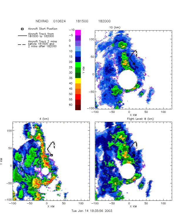
Figure 1. Constant Altitude Plan Position Indicator (CAPPI) plots at 4, 8 and 10 km for 1815 to 1820 UTC on 24 June 2001. The aircraft track during this period is superimposed on the radar data.

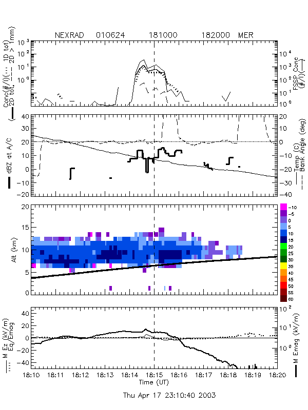
Figure 2. Microphysics, e-field and radar (MER) plot for 1810-1820 on 24 June 2001. The top panel shows cloud particle concentrations from the aircraft sensors. The second panel shows air temperature and bank angle (to indicate turns) as measured by the aircraft plus the ground-based radar reflectivity at the aircraft position. The third panel shows the aircraft altitude and a time-height display of ground-based radar reflectivity along the flight track. The bottom panel shows the electric field measured by the aircraft.

The MER and CAPPI plots were manually examined for each of the 30 days in the ABFM data set. A list of each entry into or exit from cloud was compiled with the time of the transition estimated to the nearest ten seconds. At the same time, the behavior of the cloud physics measurements was noted. A tentative relationship between these variables and the analyst's judgment regarding the presence or absence of cloud was formed. This judgment was refined by more detailed examination of each cloud boundary transition until the algorithm presented below for determining whether cloud was present was formulated.

Next, the algorithm was coded and run without manual intervention on just the ASCII data. The results were compared with the manual analysis. In most cases, the results were identical. In those cases where there were discrepancies, further analysis proved the automated algorithm to be correct. This will be discussed in the results section below.

Once the reliable method of determining in vs. out of cloud was complete, the remaining task for automated boundary detection was to incorporate some way of handling fluctuations at cloud edges to avoid rapid cycling in wispy cloud fragments at the cloud boundary. This was accomplished with a hysteresis check also described below. These two elements, cloud detection and hysteresis, compose the cloud edge detection algorithm. Comparison of the manual and automated cloud edges was used to select the appropriate hysteresis threshold.

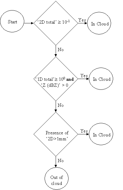
Part 2. The Cloud Presence Component

Upon examining the MER plots, it became apparent that if the Particle Measuring System (PMS) 2D Cloud Probe ‘2D total’ was > 10^-1per liter then the aircraft was in cloud. There were frequent cases where the ‘2D total’ was < 10^-1 per liter but there was cloud present. In order to diagnose these cases, the PMS 1D Cloud Probe ‘1D total’ was examined along with the radar reflectivity at the aircraft ‘Z (dBZ)’. If the 1D probe was > 10⁰ per liter and the radar reflectivity was > 0 dBZ then the aircraft was in cloud. If neither of the above indicated the presence of cloud, the presence of any large particles on the PMS 2D probe, ‘2D>1mm’, would indicate that the aircraft was in cloud. Otherwise, the aircraft was out of cloud. Because this algorithm was created for anvil and mid to high-level clouds, it is possible for a false "in cloud" reading to occur in some circumstances such as low level flight in precipitation.

The following flow chart shows the algorithm.

Part 3. Hysteresis Component

Since the goal of locating cloud boundaries for this project is to examine the variation of electric field with distance from cloud edge, it is essential to isolate true boundaries of significant clouds. Unfortunately, small wisps of cloud in otherwise clear air will be designated as "in cloud", and small gaps in otherwise solid cloud masses will be designated as "clear" by any local automated cloud detection algorithm. These designations are not erroneous, but neither are they desirable for finding the true edge of nearly continuous cloud masses.

The solution we have adopted is to only use "clean" cloud boundaries in our data set. A clean boundary is a cloud boundary with two additional constraints, called "hysteresis" constraints. There are four steps in the process. Unless all four steps are satisfied, there is no cloud edge as defined by this algorithm. In the steps listed below, a "record" refers to one line of ten-second data in a data file. Each line contains the ten second average of each of the measured variables along with the position and attitude of the aircraft and the time of day. The syntax Record(I).x is used to indicate the value of variable x in record(I) where I is the sequential record number.

Examine the current record (I) for a transition from cloud to clear or clear to cloud. A transition is present if Record(I).InCloud XOR Record(I-1).InCloud is true. InCloud is a boolean record variable that is TRUE if the in-cloud component of the algorithm is satisfied as described in the previous section.
If a transition has occurred, examine the previous 20 records to locate how many records (JMinus) back the immediately previous transition occurred. A previous transition is present at record (I- J) if Record(I-1).InCloud XOR Record(I-J-1).InCloud is true. If no transition is found, JMinus is set to 20.
If a transition has occurred, examine the next 20 records to locate how many records (JPlus) ahead the next transition occurs. Another transition is present at record (I+ J) if Record(I).InCloud XOR Record(I+J+1).InCloud is true. If no transition is found, JPlus is set to 20.
Both JPlus and JMinus must be greater than or equal to a user-selected value, H, between 0 and 10.

Selecting H = 0 turns off all hysteresis testing and locates all boundaries, however evanescent. Setting H=N assures that at least N continuous records of the same kind (in cloud or clear) exist on each side of the boundary.

For the ABFM program, the records are spaced 10 seconds apart. The true airspeed of the research aircraft ranged from 100 - 130 m/s. Thus, the value of H is approximately the length in kilometers of cloud/clear continuity required on each side of the cloud edge for that transition to be included in the analysis data set. Values of H ranging from 0 to 10 were tried on sample days. H=2 most closely matched the manual analysis of cloud boundaries. H<2 included transitions due to data dropouts and small puffs of cloud undetectable on radar. Data dropouts can occur for a variety of reasons including instrument anomalies, recording system failures, power bus transients and operator error. H>2 eliminated transitions significant enough for the analyst to list them.

Part 4. Data verification

Once the “in-cloud” rule was devised and the hysteresis concept developed, code was created and the data set was processed. A sample of part of the program output is shown in Table 1. The columns labeled C(N) contain the algorithm's evaluation of whether the aircraft was in cloud or in the clear at time N from the cloud boundary detected by the algorithm. N ranges from -5 to 5 where each unit corresponds to ten seconds of flight. This unit was selected for two reasons. First, the data were available at ten second intervals, so N corresponds to the number of records from the boundary. Second, the aircraft speed was about 100 m/s so each unit is approximately 1 Km of distance. If all of the data required to determine the presence of cloud were flagged by the automated QC process as suspect, the designation "?Clear" appears in the table.

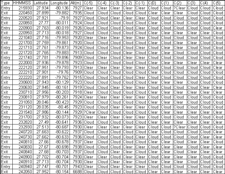
Table 1. Example of output from automated cloud-edge detection algorithm with H=0.

This was compared to the manual cloud detection spreadsheets completed beforehand. The results showed all of the manual entry/exit points had been picked up by the software as well as some additional points. These other points were examined more closely and determined to be correct. The reason for their being overlooked in the manual process was because all of the transitions missed were less than 20 seconds and many appeared near the edge of the MER plots so that they appeared to be artifacts of the plotting process. For this reason a hysteresis of 2 was chosen as the optimum one. In the full data set, the manual process found 1014 entry/exit transitions while the automated algorithm found 1269.

Part 4. Conclusion

An automated process for identifying cloud boundaries in airborne cloud physics data with accompanying ground based radar was developed and tested. It performed slightly better than manual analysis on an extensive data set from the Airborne Field Mill Program. It will permit automated analysis of the variation of electric field and radar reflectivity with distance from cloud edge. It can also be used to automate stratification of data depending on cloud presence for statistical analysis. Both of these functions are extremely labor intensive when performed manually. The automated algorithm is expected to reduce the labor required for the target analyses by more than 75%.

References

Merceret, F.J. and H. Christian, 2000: KSC ABFM 2000 - A Field Program to Facilitate Safe Relaxation of the Lightning Launch Commit Criteria for the American Space Program, Paper 6.4, 9th AMS Conference on Aviation and Range Meteorology, Orlando, Florida, 11-15 September 2000.

Merceret, Francis J. and Jennifer G. Ward, 2002: Attenuation of Weather Radar Signals Due to Wetting of the Radome by Rainwater or Incomplete Filling of the Beam Volume, NASA Technical Memorandum TM-2002-211171, April 2002, 16pp.

Short, D.A. (2000): Final Report on IRIS Product Recommendations, NASA Contractor Report CR-2000-208572, Applied Meteorology Unit, ENSCO, Inc., 1980 N. Atlantic Ave, Cocoa Beach, FL 32931, 26 pp.

APPENDIX A – Instrumentation

UNIVERSITY OF NORTH DAKOTA

CESSNA CITATION II RESEARCH AIRCRAFT

Introduction

The University of North Dakota owns and operates a Cessna Citation II aircraft (N77ND) for the purpose of atmospheric research. This aircraft type has a number of design and performance characteristics that make it an ideal platform for a wide range of atmospheric studies. The Citation II is a twin-engine fanjet with an operating ceiling of 43,000 feet (13.1 km). The turbofan engines provide sufficient power to cruise at speeds of up to 340 knots (175 m s^-1) or climb at 3300 feet per minute (16.8 m s^-1). These high performance capabilities are accompanied by relatively low fuel consumption at all altitudes, giving the Citation an on-station time of up to 4 hours or more, depending on mission type. Long wings allow it to be operated out of relatively short airstrips and to be flown at the slower speeds (140 kts/72 m s^-1) necessary for many types of measurements. The Citation is certified for flight into known icing conditions.

The cabin measures approximately five feet in diameter and more than 16 feet in length. The minimum flight crew is pilot, co-pilot and data system operator. Two additional seats are available for scientific observers or additional instrumentation specialists.

A series of structural modifications have been made to the basic airplane. These include the following: pylons under the wing tips for a variety of probes in the undisturbed air flow away from the fuselage; a heated, 5-port radome for wind measurement; and an air inlet port and manifold for air sampling inside the pressurized cabin. A summary of the operating characteristics of the aircraft is given in Table A1.

Table A1

Operating Characteristics of the Citation II

Ceiling	13.1 km	(43,000')
Endurance (plus reserves)	up to 4.5 hours
Empty Weight (including Std. instrumentation)	3888 kg	(8554 lbs)
Max Takeoff Weight	6591 kg	(14,500 lbs)
Range (not including reserves)	2500 km	(1350 nm)
Top Speed (True air speed, in research configuration)	630km h^-1	(340 kts)
Typical Sampling Speed (indicated)	80 m s^-1	(160 kts)
Fuel Consumption (Typical cruise configuration)	362 kg h^-1	(800 lbs h^-1)
Time to Climb from Sea Level to 3.0 km at Max Takeoff Weight	4 min
Time to Climb from Sea Level to 7.6 km (25,000') at Max Takeoff Weight	13 min
Time to Climb from Sea Level to 10.7 km (35,000') at Max Takeoff Weight	24 min
Takeoff and Landing Distance (most airports)	less than 1.9 km	(6000')
Total Power Available for Instrumentation	450A at 28 VDC
Research Power Available	35A 60 Hz 15A 400 Hz 160A 28 VDC

Instrumentation

The research instrumentation configuration used during the ABFM is listed in Table A2. The Instrumentation is described in more detail in Table A3. Typically, the equipment carried on any given research project will differ somewhat from the description given here. The installation of instruments provided by other investigators can be accommodated, subject to space, weight and electrical requirements. A variety of 19-inch racks are available to accommodate standard instruments. A picture of the aircraft as configured for the ABFM program is shown in Fig. A1.

Meteorology

The basic instrumentation package measures temperature, dew point temperature, pressure, wind and cloud microphysical characteristics along with aircraft position, attitude and performance parameters. The three-dimensional wind field is derived from measurements of acceleration, pitch, roll and yaw combined with angles of attack and sideslip and indicated airspeed. The aircraft parameters are supplied by an Applanix POS-AV strap-down gyro system with integrated global positioning system (GPS). Strap-down accelerometers provide lateral and longitudinal aircraft accelerations. Turbulence intensity can be derived from differential pressure transducers and accelerometer outputs. Cloud microphysical measurements are made with an array of Particle Measuring Systems probe s (FSSP, 1D-C, 2D-C) mounted on the wing-tip pylons. These probes measure concentrations and sizes of particles from one micrometer to several millimeters in diameter. In addition, there are probes to measure both liquid water content and icing rate.

For the ABFM project, an array of six electric field mills was installed on the aircraft. Four of these mills were located just aft of the cockpit and two more near the tail of the airplane. The output from these mills, when put into a solution matrix, yielded the three components of the electric field relative to the aircraft.

Remote Sensors

A forward or side-looking video camera is also used to provide a visual record of flight conditions. A Bendix-King vertical profiling forward-looking weather radar can be viewed in the cockpit and recorded on videotape.

Data Acquisition and Display

The data are sampled at various rates from 4 to 200 sec^-1. The sampling is controlled by the on-board computer system, which also displays the data in real time in graphic and alphanumeric formats while recording them on magnetic tape. The data can also be telemetered to a ground station and displayed in real time, or data may be telemetered from the ground to the aircraft. The data system is based on a project-customized windows system to allow flexibility in data acquisition and instrumentation in order to accommodate specific research demands.

Air Parcel Tracking

The data system can also run a "pointer" algorithm that can be set to track the three-dimensional advection of up to three separate air parcels. This allows the aircraft to sample in a Lagrangian frame of reference.

Field Support

When in the field, the Citation is accompanied by a mobile operations support trailer. This vehicle houses technical support facilities, including calibration equipment for on-site quality control, and computer systems. The meteorological data collected on a research flight can thus be processed and examined within a few hours.

Table A2

Summary of Measurement Capabilities as used in ABFM

State Parameters

Temperature Rosemount Total Temperature

Dew Point Temperature EG&G Cooled Mirror

Static Pressure Rosemount

Cloud Microphysics

Cloud Droplet Spectrum PMS FSSP

Cloud Particles PMS Optical Array 1D-C

Cloud Particles PMS Optical Array 2D-C

Cloud particles SPEC Cloud Particle Imager

Precipitation Particles SPEC HVPS

Liquid Water Content PMS King

Supercooled LWC Rosemount Icing Rate Meter

Air Motion and Turbulence

Horizontal, Vertical Wind Ported Radome, Applanix

POS

Attack and Sideslip Angles, Ported Radome, Differential

Airspeed Pressure Transducers

Aircraft Parameters

Heading, Pitch, Roll, Applanix POS-AV Strap-down

Ground Speed, Position, Gyro and Accelerometers with

Vertical Acceleration integrated GPS

Cabin Pressure Setra

Electric Fields

Electric Fields Six NASA Electric Field Mills

Table A3

UND Citation Instrumentation Specifications

Parameter Measured	Instrument Type	Manufacturer & Model #	Range	Response Time	Accuracy	Resolution
Temperature	Platinum Resistance	Rosemount Model 102 Probe	-65°C to +50°C	1 s nominal	0.5°C	0.03°C
Dew Point	Cooled Mirror	EG&G Model 137	-50°C to +70°C	2°C S^-1	0.5°C>0°C 1.0°C<0°C	0.03°C
Static Pressure	Absolute Pressure	Rosemount 1201F1	0 to 1034 mb	15 ms	3.1 mb	0.25 mb
Altitude	GPS	Applanix	0 to 20 km	10 msec update	0.1 km	1 m.
Attack Angle and Sideslip	Differential Pressure	Validyne P40D	34.5 mb	20 ms	0.09 mb (0.05°)	0.02 mb (-0.01°)
Indicated Airspeed	Differential Pressure	Rosemount 1221F	0 to 172 mb m^-2	10 ms	"0.55 mb (0.8 m s^-1)	0.04 mb (-0.06 m s^-1)
Heading	POS	Applanix	0-360°	10 ms update	12 arc min	6 arc min
Pitch, Roll	POS	Applanix	-90° to +90°	10 ms update	2 arc min	0.25 arc min
Vertical Acceleration	POS	Applanix	-10 to 30 m s^-2	42 ms	0.1 m s ^-2	0.01 m s^-2
Lateral, Longitudinal Acceleration	POS	Applanix	5.0 m s^-2	10 ms	0.1 m s^-2	0.002 m s^-2
Ground Speed	POS	Applanix	0 to 500 m s^-1	10 ms update	0.5 m s^-1	0.05 m s^-1
Position	POS	Applanix	90° Lat 180° Long	10 ms update	0.1 km	1 m
Liquid Water Content	CSIRO Liquid Water Detector	PMS	0-9 g m^-3	0.05 s	5%	0.005 g m^-3
Icing Rate	Vibrating Cylinder	Rosemount Model 871FA	0-0.0251 cm before recycle	7 s recycle	±.013 cm	0.003 cm
Cloud Droplet Spectrum	Forward Scattering Spectrometer Probe	Particle Measuring Systems (PMS) FSSP-100	0.5-47mm	4 Hz sampling	-	0.5-3.0mm variable
Cloud Particles	Optical Array Probe 1D-C	PMS OAP-230X	20-600 mm	4 Hz sampling	-	20 mm
Cloud Particles	Optical Array Probe 2D-C	PMS OAP-2DC	30-960 mm	4 Hz sampling	-	30 mm

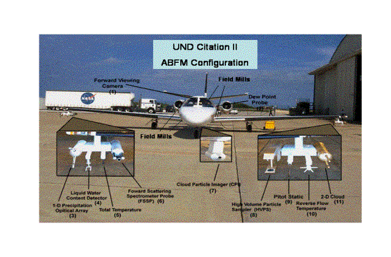
Figure A1. The UND citation with LLCC/ABFM instrumentation

APPENDIX B – Weather Radar

Two weather radars were used in this project, the National Weather Service WSR-88D (NEXRAD) at Melbourne, Florida and the Air Force WSR-74C at Patrick AFB, Florida. Except in a few cases where the aircraft was in the cone of silence of one of the radars, or where attenuation due to precipitation was a concern, the two instruments provided equivalent data.

The NEXRAD is a ten cm Doppler radar located at 28.11N and 80.65W at an elevation of 35 ft. NWS/MLB personnel recorded full volume scan data specifically for the ABFM program in real time on a dedicated 4mm DAT system supplied by the Applied Meteorology Unit. These data were processed at NCAR using custom software to translate them to a 1x1x1 Km three-dimensional grid of reflectivity. The gridded data were used in this study. The beam width and scan strategy for this radar are described in Short (2000). All missions flown during the ABFM field program were within 200 Km of the radar. Attenuation of the radar signal due to rainfall on the radome or between the radar and the aircraft was not significant at any time for this radar.

The WSR-74C is a five cm conventional radar located at 28.26N and 80.66W at an elevation of 65 ft. Eastern Range Technical Services Contractor personnel recorded full volume scan data specifically for the ABFM program in real time. These data were also processed at NCAR using custom software to translate them to a 1x1x1 Km three-dimensional grid of reflectivity. The gridded data were used in this study. The beam width and scan strategy for this radar are also described in Short (2000). All missions flown during the ABFM field program were within 200 Km of the radar. Attenuation of the radar signal due to rainfall on the radome or between the radar and the aircraft was significant at times for this radar (See Merceret and Ward, 2000, for a complete discussion of wet radome attenuation). When attenuation was not negligible, the data were not used.