The Decay of Electric Field in Anvils:

Observations and Comparison with Model Calculations

J.E. Dye¹, W.D. Hall¹, J.C Willett², S. Lewis¹, E. Defer³, P. Willis⁴, D.M. Mach⁵,

M.G. Bateman⁵, H.J. Christian⁵, C.A. Grainger⁶, J. Schild⁶, and F.J. Merceret⁷

¹ NCAR PO Box 3000, Boulder, CO 80307; ² PO Box 41,Garrett Park MD; ³ National Observatory of Athens, Athens, Greece; ⁴ NOAA/Hurricane Research Div., Miami FL; ⁵ NASA MSFC, Huntsville AL; ⁶ Univ. of No. Dakota, Grand Forks ND, ⁷ NASA/KSC, Kennedy Space Center, Florida

ABSTRACT: Airborne measurements of electric field and particle size distributions made in anvils of active and decaying thunderstorms near Kennedy Space Center, Florida coordinated with simultaneous radar observations are presented. The observations in conjunction with a simple model are used to examine the decay of electric field in anvils.

INTRODUCTION

Natural and triggered lightning pose a threat to the launch of space vehicles and also personnel at Kennedy Space Center and other launch sites. The Airborne Field Mill Project (ABFM) was conducted during June 2000 and 2001 to examine the strength and decay of electric fields in anvils, layer and debris clouds and how they are related to microphysics and radar structure to better understand when hazard from lightning might or might not exist. [Dye et al., 2002]. The airborne observations were made from the Univ. of No. Dakota Citation II jet aircraft and were coordinated with radar coverage from the Patrick Air Force Base WSR74C 5 cm radar and the Melborne NEXRAD 10 cm radar. The vector electric fields were measured using a set of 6 field mills as described in Mach and Koshak, this conference.

EXAMPLE RESULTS FOR JUNE 13, 2000

Fig. 1 shows measurements made on June 13, 2000 for a 7 minute period (~50 km of flight track). The Citation investigated this anvil for over 3 hours, first with lightning present and then for 2 hours after the last lightning. This pass at 11 km, –40 C, was east to west across the anvil

Figure 1. Top Panel: Time history of Particle concentrations measured by the following instruments: PMS FSSP (1 to 48 mm), light, solid line = total conc. on right scale; PMS 2D-C (30 mm to ~3 mm), bold line = total conc., dashed line = conc. >1 mm on left scale; PMS 1D-C (15 to 960 mm), dotted line = total conc. on left scale. Middle panel: Radar reflectivity curtain above and below the aircraft from NEXRAD radar at Melborne FL, bold line = aircraft altitude. Bottom panel: Vertical component of the electric field, Ez, bold line on left on a linear scale, and the resultant vector field, Emag, light line on right on a log scale.

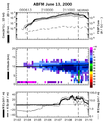
while lightning was occurring in the storm core 25 to 40 km to the south. The maximum reflectivities encountered during this pass were 15 – 20 dBZ from 2107 to 2108:30.

PARTICLE OBSERVATIONS

The microphysical observations were made with five different instruments that spanned particle sizes from a few microns to about five centimeters, thus from frozen cloud droplets to very large aggregates. Measurements from an icing detector showed no evidence of supercooled water in the example below or any other anvils investigated. All particles discussed below are ice.

The measurements of Fig. 1 are representative of anvils studied at altitudes of 8 to 11 km (roughly -20 to –45 C). The concentrations in all size ranges increase as the aircraft moves into higher reflectivities, but usually larger increases occur for particles in the size range of 100 to ~500 mm than for particles >1 mm size. In regions with strong electric fields slightly downwind of storm cores there is a surprising degree of consistency in particle size distributions from storm to storm. The concentrations from 2108:00 to 2108:30 in Fig. 1 and Fig. 2 below are typical of those observed in other thick anvils near the storm core with electric fields >20 kV/m.

Figure 2 illustrates the changes in particle concentration and area size distributions for four 30 s intervals during the anvil pass in Fig. 1. At the edge of the anvil the number distribution is almost flat from 100 to 1000 mm, but as the aircraft moves into the thicker part of the anvil the concentration of particles in the 100 to ~500 mm increase by a factor of ~50. During this same period the concentration of >1 mm particles increases by a factor ~3.

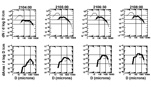
Figure 2. Top panel: Concentration size distributions (30 sec averages) for the indicated initial times during the Citation pass shown in Figure 1. Bottom panel: Area size distribution for the same 30 sec time periods. Light line on the left side of each plot -- FSSP (off scale for area plots); Bold line – 2D-C; light line on right of each plot -- SPEC High Volume Particle Spectrometer, HVPS, (~400 mm to ~5 cm range).

ELECTRIC FIELD OBSERVATIONS

Likewise electric fields are much weaker near the edges than in the central anvil or near the storm core. As in Fig. 1, the electric field is <3 kV/m for reflectivities <5 - 10 dBZ in edges of the anvil followed by a relatively abrupt increase in electric field as the aircraft flies into greater reflectivities in denser parts of the anvil or near the storm core. The electric field measurements show more variability and often increase much more abruptly than the increase in particle concentrations. The complex nature of the electric field structure and changes of polarity even when flying at constant altitude suggest that the charge distribution in these anvils is not a simple uniform layering of charge.

Strong electric fields (>10 kV/m) are associated with regions of reflectivity above the freezing level ³10 dBZ, but reflectivity >10 dBZ does not necessarily indicate strong fields. In strong electric fields particle concentrations are high in all size ranges and greater than in regions with weak (<3 kV/m) electric fields. Bateman et al., this conference, discuss the correspondence between electric field and reflectivity and investigate reflectivity parameters that might be used as possible indicators of the presence of strong electric fields.

PARTICLE SIZE DISTRIBUTIONS AND ELECTRIC FIELD DECAY

Willett and Dye (this conference) use a simple model to calculate electric-field decay times based on observed particle size distributions. The model assumes that a given size distribution is uniform everywhere in the model anvil and that it remains constant during the decay of electric field. This is not strictly correct, but it provides an upper bound on what might be expected. A "high-field limit" is identified, for ambient field intensities greater than about 1 kV/m, in which the model field decays linearly with time; and a decay time scale, t_E, is defined as the time required for the cloud field to decay to zero from an arbitrary initial value of 50 kV/m. t_E is found to be proportional to the particle effective electrical cross section (area), integrated over the size distribution. See Willett and Dye for more details.

Figure 2 displays the area size distributions for this case. t_E for the 4 time periods of Figure 2 is 340, 1256, 2656 and 5963 s, respectively. t_E increases by a factor of almost 20 from the edge to the central part of the anvil.

In Fig. 2 the area distributions, which control t_E, show a peak near 1 mm in the edge of the anvil, but as the aircraft moves into the central anvil, the area distribution becomes broad with a mode from 0.2 to 2 mm. In this case (and other cases we have examined to date) as the aircraft moves from the edge toward the central part of the anvil the largest increase in particle concentrations are of the 0.2 to 1 mm size particles. The results show this size range to be dominantly responsible for the increases in calculated electrical decay times.

COMPARISON OF CALCULATED AND OBSERVED DECAY TIMES

After lightning had ceased, passes were made into the wind from the downwind tip of the anvil into higher reflectivity in the remnants of the storm core. The southern most part of two of these passes are depicted in Fig. 3. The maximum reflectivities from 2253 - 2258 were 14 to 17 dBZ and 12 to 15 dBZ for 2324 – 2330. The maximum electric fields observed during the first pass were 39 kV/m at 2253:30. During the second pass the electric fields had decreased to a maximum of 1.5 kV/m at 2253:30, a decay of 37.5 kV/m in 32 min (1920 s). By comparison the maximum in the calculated E time scale, t_E, for the decay from 50 kV/m was 1711 s for the period 2253:30 to 2254:00. Using this time scale we calculate via equation 5) of Willett and Dye, this conference, a time of 1275 s for the electric field decay from 39 to 1.5 kV/m based on the 30 s average particle size spectra observed at 2253.

The observed decay times are longer than those calculated. However, the model assumes uniform microphysics in the anvil and during the entire decay. The reflectivity below the aircraft (Fig. 3) was 5 dBZ or more greater at 7 km than at 9 km, the aircraft altitude. Clearly the largest particles were more numerous below the aircraft and quite probably the intermediate sized particles as well. Measurements in this anvil (Figs 1 and 2) and other anvils show that as reflectivity increases, concentrations and area in all particle size ranges also increase, especially from 0.2 to 1.0 mm. For the 30 s averages for 2105 and 2108 (Fig. 1) t_E increased from 1256 to 5963 s, almost a 5 fold increase as a result of increased particle area at intermediate sizes (See Fig. 2). The corresponding reflectivity increase was ~5 dBZ. It seems likely that if particle observations were available at 7 km for this anvil, they would yield electric field decay times more than enough to account for the difference between observed and calculated values discussed above. None-the-less, this comparison of calculated and observed electric field decay time shows that the decay times calculated in the model for this anvil are roughly comparable to those observed.

A similar comparison for June 14, 2000, a case where the aircraft flew in the greatest reflectivities in the decaying anvil, shows the observed times for decay bracket those calculated.

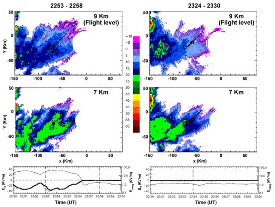
Figure 3: CAPPIS at 9 and 7 km for 2 periods with 9 min of aircraft track overlaid. Squares show track start. Lower Panels: Measured vert. field, Ez, (bold line, left scale) and magnitude of total field, Emag, (thin line, logartithmic right scale) for 2250 - 2300 and 2320 – 2330.

CONCLUDING REMARKS

Observations of particle spectra and electric fields in anvils in regions with strong electric fields show consistency of particle concentrations in all size ranges from storm to storm. These observations in combination with model calculations of electric field decay in a simplified anvil (Willett and Dye, this conference) show that the particle size distribution controls the decay time of electric field in these anvils. Particles of 0.2 – 1 mm size are predominantly responsible for changes in decay times along and across the anvils. As air containing ice particles moves out from the convective core into anvils and downwind, the particle spectra change due to sedimentation, mixing and evaporation and the time for decay of the electric field dramatically decreases.

ACKNOWLEDGEMENTS; We gratefully acknowledge support from the National Aeronautics and Space Administration (Kennedy Space Center) and the National Reconnaissance Office, the help and encouragement of John Madura and Phil Krider, and graphics work of Kris Conrad.

REFERENCES

Bateman, M.G., D.M. Mach, S. Lewis, J.E. Dye, E. Defer, C.A. Grainger, P.T. Willis, H.J. Christian, F.J. Merceret, 2003: Comparison of in-situ Electric Field and Radar Derived Parameters for Stratiform Clouds in Central Florida, This Conference.

Dye, J.E., W.D. Hall, S. Lewis, E. Defer, G. Dix, J.C. Willett, C.A. Grainger, P. Willis, M. Bateman, D. Mach, H. Christian and F.J. Merceret, 2002: Microphysical Properties and the Decay of Electric Fields in Florida Anvils, presented at AGU Fall Meeting, San Fransisco, CA, Dec 2002. Abstract in EOS Trans. Amer. Geophys. Union.

Mach, D. M. and W. J. Koshak, 2003: General Matrix Inversion Technique For The Calibration Of Electric Field Sensor Arrays On Aircraft Platforms, This Conference.

Willett, J.C. and J.E. Dye, 2003: A Simple Model to Estimate Electrical Decay Times in Anvil Clouds, Proc. This Conference