BRIEF DESCRIPTION OF THE MICROPHYSICAL INSTRUMENTS USED FOR ABFM

J. Dye
October 7, 2002

A number of different probes were used to measure particles during the ABFM project. The following is a very brief overview of the different instruments, how they performed in general and some issues to consider when examining the time series plots of particle concentrations which exist on the NCAR ABFM Web Site.

The instruments used were:

1) PMS Forward Scattering Spectrometer Probe (FSSP)
Nominal range 3 to ~50 microns in 15 bins The FSSP sizes and counts particles by measuring light scatter in the forward direction. The voltage pulses produced are sized and sorted into 15 bins in a pulse height analyzer. The instrument was designed to count and size cloud droplets which are spherical and water. In recent years some researchers believe that the FSSP output gives a reasonable idea of total concentration in clouds wholly composed of ice, but not mixed phase. We include the total concentration from the FSSP as a measure of the smallest ice in the cloud. Uncertainty in the total concentration measurement is unknown, but could be a factor of two or perhaps more. Paul Field has recently shown that artifacts can be produced by breakup of ice particles colliding on the tips of the FSSP, but estimated that the uncertainty is probably less than a factor of two.

ISSUES: The FSSP often has noise in the first bin or two, because the threshold for the first bin is set close to the signal noise level (which can be variable in different conditions). Hence out of cloud you might see some response from the FSSP even though the 2D shows nothing. I have seen this for a couple of days in 2000 and in 2001. Additionally, during the early part of the May/June 2001 campaign there was an intermittent power supply that sometimes functioned and sometimes not.

For more detailed description of the FSSP go to:

2) Particle Measuring Systems (PMS) 2D-Cloud Probe (2D-C)
Range 33 um to ~1 mm on the UND Citation The 2D-C produces shadows of particles passing through a collimated laser beam by recording the time sequence of diodes of a 32 element diode array which are shadowed by passage of the particle. By scanning the array at a speed propotional to the aircraft true airspeed, an image of each particle is generated. The sample volume is size and true airspeed dependent, and must be accounted for in processing. Substantial processing must occur to determine concentrations and size distributions. The probe has 2 buffers which allows one buffer to collect data, while the previously filled buffer is downloaded. On the UND system 4 buffers/sec can be recorded.

ISSUES: In both 2000 and 2001 there were some power supply problems, meaning loss of data. Frequently every other buffer is difficult to read and sometimes lost. This was particularly true in June 2001 for all flight days after the lightning strike on 10 June 2001. On occasion when the Citation was in strong E fields the probe tips apparently go into corona. When this happens artifacts are generated and the timing words which are essential for interpreting the data record are corrupted. The data can not be recovered for those periods. These artifacts were fairly common during flights in which high fields were encountered, but did not always happen when the fields were strong. Undersampling of particles in the lower range of the 2D probe is well known. It is a result of poor electronic time response and probability of detection when particles are near or only a little larger than the size of the elements of the diode array. Concentrations of particles for sizes less than ~100 microns are underestimated and sometimes this portion of the size distribution is not included in size distributions. We have included them for completeness, but the absolute concentrations should not be trusted.

For further description of operation of the 2D probe go to:

For samples of 2D particle images for each flight day of the June 2000 or May/June 2001 campaign go to:

2D samples

Select the year of interest, 2000 or 2001, and then the flight day. This brings up a list of images from that flight. One out of every 100 buffers recorded by the 2D is shown.

3) PMS 1D-Cloud Probe (1D-C)
Range ~20 to 600 microns
The 1D probe, like the 2D probe, has a 32 element diode array. But instead of scanning the array and recording occulted diodes, the 1D electronics determines the maximum number of diodes occulted by each particle. This information is sorted and counted into different size bins of a pulse heightt analyser. The first and last diode are used to determine if a particle is wholly in the beam. Thus functionally only 30 diodes are used for sizing. Particle size distribution are recorded but without images of the particles.

ISSUES: We only recently started processing the 1D data, so we are not fully aware of any issues. Like the FSSP, there can be noise in the first couple of size bins, but so far I have not noticed this in the ABFM measurements. My impression is that for the ABFM project, the 1D probe may be the most reliable indicator of when the aircraft enters and leaves cloud. Like the 2D, under sampling of particles in the lower range of the 1D probe is well known. It is a result of poor electronic time response and probability of detection.

For more information on principles of operation of the 1D probe go to:

1D Probe

The above description is for a probe with a 60 element array whereas the Citation probe has only 32 elements.

4) King Liquid Water Sensor
The King liquid water probe maintains a wire element at a constant temperature and senses the power necessary to keep the element at a constant temperature. Because heat loss occurs in clear air as well as cloud, a "dry" term correction must be made.

ISSUES: Measurements by others in clouds containing only ice particles (no liquid particles) have shown that this sensor does respond fractionally to ice as well as water. Thus, it's measurements should not be used as a measure of the supercooled liquid water in our anvil clouds.

For more information on this instrument go to:

King LWC

5) Rosemount Ice Detector
This sensor is a small cylinder of a couple centimeters length and a few millimeters diameter which when in supercooled water becomes iced. A magnetostriction circuit determines the change in resonant frequency of the cylinder and the signal output is proportional to accumulated ice mass. When a preset threshold is reached the cylinder is heated to remove any accumulated ice and a new icing cycle is begun. This is the best measure we have for the possible presence of supercooled water in ABFM anvils.

ISSUES: At times spikes are observed in the signal. These are perhaps due to graupel or other large ice particles impacting on the cylinder.

For more information on this instrument go to:

Ice Probe

6) SPEC Cloud Particle Imager (CPI)
This is a relatively new instrument which in the hot, humid Florida environment required a lot of attention. When operating properly it produces spectacular images of ice particles and water drops. The CPI uses two crossed continuous laser diodes to sense when a particle is in the intersection of the two beams. Then a 30 mW laser diode is pulsed at ~20 nanosec to capture the image of the particle (and any others in the path) on a 1024 x 1022 CCD array. Each element of the array is ~2.5 microns, so particles in focus show great detail including particle habit and any evidence of riming.

ISSUES: The sample volume of the CPI is small, roughly 2.5 x 2.5 mm square. Thus it captures images primarily in the range of ~20 microns to a few hundred microns, because the probability of triggering on larger ones is so small. Additonally this instrument is sufficiently new that so far we are not able to determine concentration independent of other measurements. Also processing and analysis of the data are extremely time consuming. For ABFM we are using the measurements primarily for the images and information on particle types encountered during selected flights.

For more information on the CPI go to:

CPI

7) SPEC High Volume Precipitation Spectrometer (HVPS)
This probe was designed to greatly increase the sample volume for larger particles. It's operation is somewhat similar to that of the 2D but is much more complex. It uses two linear arrays of 256 elements each with each element corresponding to 200 microns width in the sample volume. Thus, the entire width of the beam is almost 5 cm, meaning that particles as large as 5 cm can be imaged. The scan rate for sampling the array is slaved to the true airspeed so that the resolution along the line of flight is roughly 400 microns for airspeeds under 96 m/s.

ISSUES: During the June 2000 campaign the HVPS worked poorly, apparently due to misalignment of optics. However, during the Feb. 2001 and the May/June 2001 campaigns the HVPS worked very well and gives us excellent information on the large particles of the spectrum. In principal, determination of the sample volume and hence concentration should be relatively straightforward, but only a few investigators have used the HVPS so it is hard to address uncertainties at this time. In general there is relatively good agreement between the 2D and the HVPS in the crossover region of the two instruments. Like the 2D and 1D probes, the HVPS undersamples the small end of it's size range because the probability of detection is reduced when the particle size is not significantly larger than the distance between the elements of the array.
For more information on the HVPS go to:

HVPS

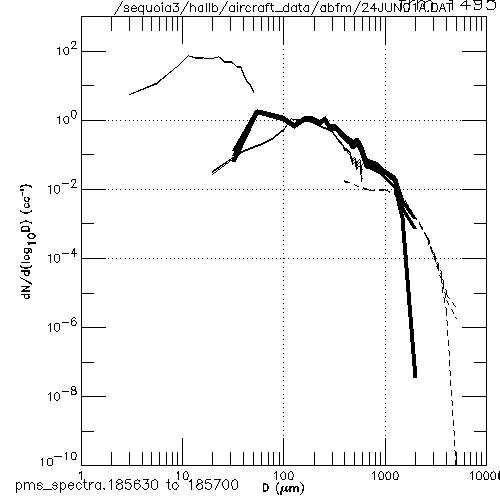
EXAMPLE of a Particle Size Distribution
Combined from measurements of the FSSP, 1D, 2D and HVPS for June 4, 2001 from 2029:30 to 2030:00.

solid, light line in upper left is from the FSSP
solid, BOLD line is from the 2D
solid, light line near the 2D line is from the 1D
dashed line is from the HVPS

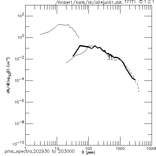
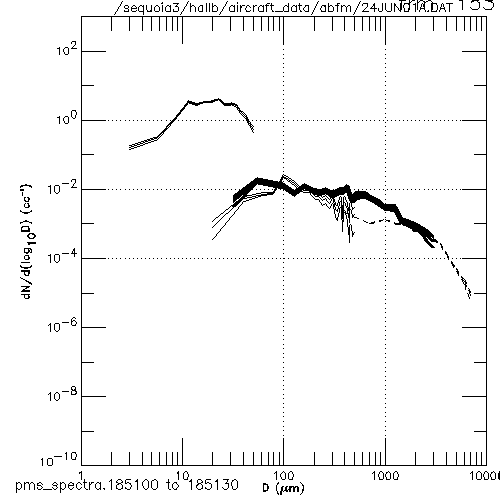
Statistical Uncertainty in Particle Concentration Measurements

The following three particle size distribution plots for the 24June2001 case span a range of particle concentrations encountered during ABFM. The first case (1851:00) is one with relatively low concentration near the radar edge of the anvil, the second one (1852:30 is with intermediate concentrations and the last one (1856:30) is with large concentrations, particularly for sizes from 100 to 1000 microns. These three plots show statistical uncertainty in particle concentrations from the different particle probes as a result of counting statistics. The uncertainty was calculated following Cornford (1967) and is based on poisson statistics. There are three traces for each instrument. The middle line is the best estimate, and the upper and lower lines (when distinguishable from the middle line) are the upper and lower 95% confidence limits. In many cases for our distributions the 95% confidence limits are no wider than the line width. Uncertainties appear mostly at the upper and lower size limit of each instrument where the number of counts are smaller.
NOTE: These are the uncertainties due to counting statistics. There are additional sources of uncertainty inherent in each instrument.

The uncertainty of the concentration measurements in any size interval (instrument defined bin limits) of the distribution is
1 +/- [1/sqrt(Ci)], where Ci is the number of counts measured by a given instrument in the size interval i. For example, if the measured number of counts in a given size interval is 100, the 95% confidence limits of that measurement are 110 to 90, ie. 100(1 +/- [1/sqrt(100)]).
If the number of counts is 10, the uncertainty range is 13.2 to 6.8. If only 1 particle is detected in a give size interval, the 95% confidence limits range from 2 to 0.

REF: Cornford, S. G., 1967: Sampling errors in measurements of raindrop and cloud droplet size concentrations. Meteor. Mag., 96, 271-282.

An example for June 24, 2001 from 1851:00 to 1851:30 -- low concentrations

An example for June 24, 2001 from 1852:30 to 1853:00 -- intermediate concentrations

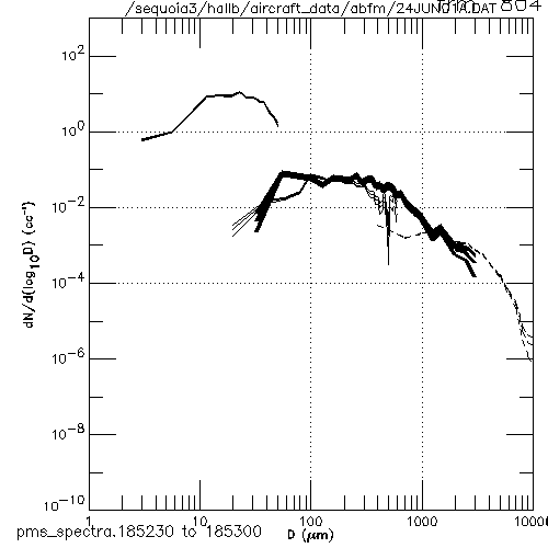
An example for June 24, 2001 from 1856:30 to 1857:00 -- large concentrations