Tutorial example: global orographical flow

The example is based on the orographic flow (Smolarkiewicz et al. 2001) of a shallow fluid on a rotating sphere. It was proposed by Williamson et al. (1992) for evaluating the accuracy and efficiency of numerical methods for global-scale dynamics and has become a benchmark in the field. Its original formulation is in terms of the shallow water equations. Here, we extend this problem to a continuously stratified 3D Boussinesq fluid while keeping other flow parameters consistent with the benchmark. We use the Boussinesq option of the anelastic model to enable meaningful comparisons of the three governing systems,

.

In this manner, we can quantify the effects of the non-Boussinesq baroclinicity and finite speed of sound relative to the truncation errors of finite-difference approximations. We anticipate these results would extrapolate to similar comparisons of the anelastic and fully compressible Euler equations.

and the corresponding thermally balanced state

where ϒ̂_e(r') = ϒ_o[1 + r'N²/g], and the Brunta-Vaisala frequency N = 10^-2 s^-1. Here r, R, Psi, and Omega denote, respectively, the radial component of the vector radius, sphere's radius, latitude, and angular velocity of the planetary rotation. Also, r/R, and r'=r-R. The conical hill with height 2 x 10³ m and base radius Pi/9 (in terms of lat-long) is centered at (Lambda, Psi) = (3Pi/2,Pi/6), where Lambda is the longitude. The globe is covered with a uniform spherical mesh with nx x ny = 128 x 64 grid intervals (no grid points at the poles) and the H = 8 x 10³ m deep atmosphere is resolved with nz = 20 uniform grid intervals. The time step Dt = 7.2 x 10³ s.

below is a set of conditions specific for this test case:

      parameter (n=128,m=64,l=21)                ! grid dimensions
      parameter (dx00=1.)
      parameter (dy00=1.)
      parameter (dz00=500.)
      parameter (dt00=600.)

      parameter (nt=1440,noutp=288,nplot=288,nstore=720,nslice=0)
      parameter (iwrite=1,iwrite0=0,irst=0)

      parameter (icyx=1)
      parameter (icyy=0)

      parameter (implgw=1,isphere=1,icylind=0,icorio=1)

#define SGS 0      /* 0=NO DIFFUSION, 1=OLD DISSIP, 2=DISSIP AMR      */
      parameter (ivs0=0)                          ! Viscous/Inviscid model
      parameter (itke0=0,itke=ivs0*itke0)         ! Smagorinsky/TKE SGS model
      parameter (ichm=0,nspc=3)              ! chemical spices
      parameter (imrsb=0)

ccccccccccccccccccccccccccccccccccccccccccccccccccccccccccccccccccc
create environmental profiles (use subroutine tinit_i)            c
c-----------------------------------------------------------------c
c---> u00 - wind constant; x component, profile U       (m/s)     c
c---> v00 - wind constant; y component, profile V       (m/s)     c
c---> st  - stability parameter; inverse scale height   (m^-1)    c
c---> u0z - vertical wind shear dU/dz                   (s^-1)    c
c---> v0z - vertical wind shear dV/dz                   (s^-1)    c
ccccccccccccccccccccccccccccccccccccccccccccccccccccccccccccccccccc
      data     u00,    v00,     st,    u0z,    v0z
     $        /20.0,   0.0, 1.0e-5,  0.e-3,  0.e-3/

ccccccccccccccccccccccccccccccccccccccccccccccccccccccccccccccccccc
create mountain
c-----------------------------------------------------------------c
c     amp  - maximum height of mountain [m]
c     xml  - zonal scale of mountain [m] or [radians]
c     xml0 - zonal shift from the domain center [m] or [radians]
c     yml  - meridional scale of mountain [m] or [radians]
c     yml0 - meridional shift from the domain center [m] or [radians]
c     angle- angle to skew the mountain ridge [radians]
ccccccccccccccccccccccccccccccccccccccccccccccccccccccccccccccccccc

      common/gora/ xml,yml,amp,xml0,yml0,angle
      data amp,xml,yml,xml0,yml0,angle/2.e3,2*.34906585,3*0./

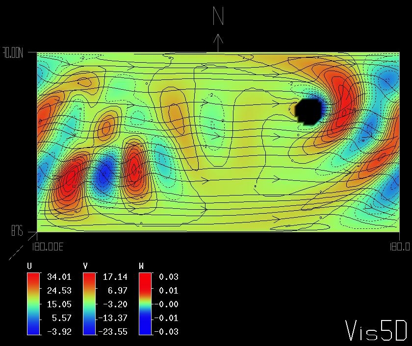
Figure 1 shows the pattern of vertical and meridional velocity components after 15 days of simulated zonal flow of a stratified Boussinesq fluid past a large hill (consistent with the linear solution of Grose and Hoskins 1979; cf. their Fig. 3a) using the semi-Lagrangian implicit variant of the model discussed above. The flow parameters are

Figure 1. Ncar Graphics plot. Planetary wave propagation on a sphere. Contours show patterns of (a) vertical and (b) meridional velocity components in m s-1, with imposed flow vectors, at 4 km after 15 days of simulation. Contour maxima (cmx), minima (cmn), and intervals (cnt) are shown in the upper-left corner of each panel. Negative values are dashed, and zero contours are omitted. The mountain is illustrated with thick solid circles. Maximum vector lengths (here identical) are shown in the upper-right corner of each plate.

Figure 2. Vis5D plot corresponding to Figure 1.

Grose, W. L., and B. J. Hoskins, 1979: On the influence of orography on large-scale atmospheric flow. J. Atmos. Sci.,36, 223.234.

Smolarkiewicz, P. K., L. G. Margolin, and A. A. Wyszogrodzki, 2001: A class of nonhydrostatic global models. J. Atmos. Sci., 58, 349.364.

Williamson, D. L., J. B. Drake, J. J. Hack, R. Jakob, and P. N. Swarztrauber, 1992: A standard test set for numerical approximations to the shallow water equations on the sphere. J. Comput. Phys.,102, 211.224.