The model source code for Version 3 contains more than 220 subroutines and about 55500 lines of code including comments. It is written to be portable to many platforms and so is generally standard in terms of its Fortran and it is self-contained in that it does not require additional libraries to run.
Since the code was developed originally for efficiency on a Cray, it is written
to vectorize as efficiently as possible. A vectorized loop on these machines
is many times faster than an unvectorized one. To achieve this, the inner do-loops
are often in a horizontal direction to both maximize the vector length and to
reduce the possibility of index dependencies that would inhibit vectorization.
This is not optimal for non-vector machines with small cache because it can
lead to more frequent memory calls as these loops are executed as opposed to
the case where the inner loop is short. However, in practice the code runs well
on RISC/cache machines.
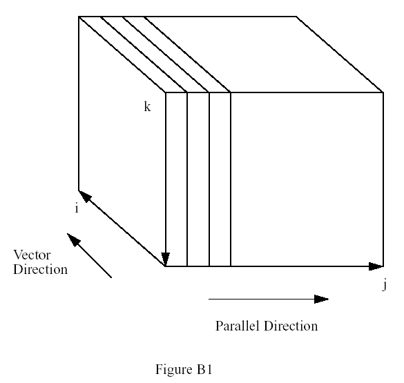
Even though most of the physics operates on vertical columns, the physics routines take a whole north-south slice (see next section) so that vectorization can be done over the I-index (south-north) (Fig.B1).
Again because of the development on shared-memory parallel Cray processors,
the code is structured to make efficient use of this. Use of multiple processors
in parallel speeds up a task by an amount depending on the parallel efficiency.
Typically for MM5, eight processors can speed up the job by a factor of six.
Although this costs more in CPU time it has benefits in real-time forecast applications
in getting the forecast out quickly, and sometimes the charging algorithm favors
efficiently parallelized jobs, as they may get the benefit of special low-cost
queues. The code also contains parallelization directives for SGIs and can in
principal be parallelized on any multi-processor workstation.
To achieve efficient parallelization outer do-loops are often distributed across processors. For instance, there are several parallel J-loops in the SOLVE routine. J is the west-east horizontal index, and by having the outer loop over this index the physics calculations are done in north-south vertical slices. When a J-loop is multi-tasked each value of J goes to a different processor, so that each operates on a different north-south slice. As processors finish the calculations in their slice they take the next available one. It can be seen that the code has to be written carefully to allow this to work, and essentially each J-slice’s calculations must be independent of the results generated by other slices.
Multi-tasked sections of code have a clear distinction between shared and private (or local) memory. Shared memory is seen by all the processors, while private memory is seen only by a single processor as each processor has its own copy of these arrays. Often the multi-tasking preprocessor is able to decide which variables are shared or private but some declarations are required, particularly for variables passed into subroutines within a multi-tasked loop. In general scalars and arrays that are constant in the parallel region (read only) should be shared, while those that do change their value (are written to) should be private. The major exception to this is an array with an index corresponding to the multi-tasking index (e.g. a J index in a DO J multi-tasked loop). These arrays have to be shared and special care is required if the array is written to. It is safest to avoid references to J+1, J-1 etc. elements within a multi-tasked J loop. The computation will execute the J loop in essentially random order, so no dependence on results from other J-slices should exist.
Common blocks within parallel sections of code also have to be treated carefully. If each task needs its own copy of a common block, such as for storing temporary variables that are not dimensioned by the tasked loop index (usually J), there is a Cray command
CDIR$ TASKCOMMON common-block-name
that accomplishes this. A new standard for parallel directives, recognized by many vendors now, is OpenMP. The directive for the above in OpenMP looks like
c$omp threadprivate (/common-block-name/)
On older SGI compilers (without OpenMP) this is achieved by a special -Xlocal declaration in the load options. Without such directives all tasks will attempt to use the same memory space leading to unpredictable results. Note that this is rarely required in MM5 since most common blocks contain domain-wide variables and constants. However, the Burk-Thompson and Gayno-Seaman PBL schemes use common blocks for storing temporary values to pass between its own subroutines, as do the Noah land-surface model and the RRTM radiation scheme.
Parallelization is implemented by placing a special directive ahead of the parallel loop. For example, the following loop parallelizes over J,
cmic$ do all autoscope
c$doacross
c$& share(klp1,qdot,wtens,il,jl),
c$& local(i,j)
c$omp parallel do default(shared)
c$omp private(i,j)
DO J=1,JL
DO I=1,IL
QDOT(I,J,KLP1)=0.
WTENS(I,J,KLP1)=0.
ENDDO
ENDDO
where the cmic$ represents a Cray directive and c$ represent SGI
directives, and c$omp represent OpenMP directives. Note that these appear as
comments to a Fortran compiler and only have special meaning to the parallel
preprocessors.
Perhaps the most nonstandard aspect of the code is the use of Cray pointers
which are now supported on most platforms. In the model these are used to allow
the code to operate on multiple domains without the need for an additional array
index to identify the domain. When the code is doing calculations for a given
nest, the pointers give the locations in the memory of all the arrays associated
with that nest. Thus subroutines using these arrays, such as UA (a 3D array
of x-direction wind component), have to have a pointer statement as follows.
POINTER ( IAUA, UA(MIX,MJX,MKX))
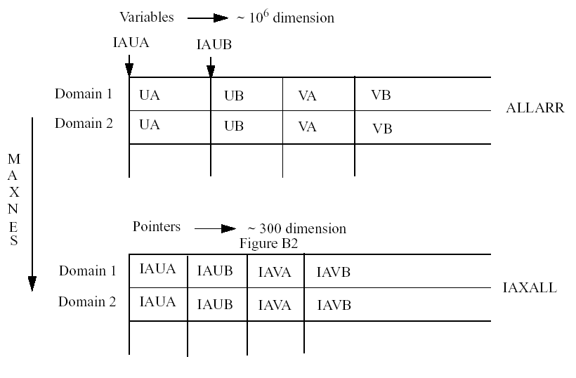
IAUA is an address locating the first element of UA which is dimensioned by parameters MIX, MJX and MKX. The model typically uses about 300 such addresses to locate all the information on a given nest. These 300 variables representing 0-dimensional scalars to 4-dimensional arrays are actually stored end-to-end in two super-arrays, one for reals (ALLARR) and one for integers (INTALL) (Fig. B2). There are also additional super-arrays for FDDA. The pointers locate the starting position of each variable in the super-array. This array is dimensioned by the sum of all the array sizes, which may reach a few million, as its first index and by the number of domains as its second index. Routine ADDALL, called once at the beginning of the simulation, calculates all these addresses based on the sizes of the arrays, gets their absolute addresses with the LOC function, and stores these in a 2D array (IAXALL) dimensioned by about 300 and the number of domains.
Each time the model calculations shift from one domain to another the addresses in the pointers, such as IAUA, have to be changed by a call to routine ADDRX1C which has the new domain number as an argument. Sometimes information for two domains is needed at once, such as when a nest feeds back to the coarser mesh, and ADDRX1N is used to locate the addresses for the second domain. These routines take the relevant addresses from IAXALL and put them into common blocks such as /ADDR1/ (see below), overwriting the common blocks each time the routines are called.
COMMON/ADDR1/ IAUA, IAUB, IAVA, IAVB, IATA, IATB, IAQVA,...
There are several common blocks of pointers, and these are passed to various routines together with the pointer statements. The use of pointers allows the routines not to require domain number specifiers. Alternative methods would either require a large number of EQUIVALENCE statements, or equivalencing through passing a large number of arguments into certain routines.
Distributed-memory machines are becoming increasingly common. These machines can run a gridded domain by distributing the grid across a number of independent processors which all only calculate and store information for a sub-area of the grid. At various points during the calculation there needs to be communication between processors, but the coding has to minimize these to maintain efficiency.
In 1998, in release 2.8, we added a capability for MM5 to run on distributed-memory machines. This involves several code pre-compilation steps, and uses mostly the same code as the standard MM5, with `ifdef MPP' being used to isolate specific differences. The pre-compilation involves two stages. In the first using FLIC (Fortran Loop and Index Converter), DO loops are replaced by generic FLIC directives and other areas of the code are modified to allow for distributed memory. In the second stage RSL (Run-time System Language) commands are inserted which is a high-level language built on the low-level MPI standard for message passing. This leads to an automated code conversion which is run as part of the "make" process when MPP options are selected.
John Michalakes (Argonne National Laboratory) has developed FLIC and RSL and applied them to MM5. The resulting extension of MM5 to these platforms is proving to make efficient use of multiple distributed processors on machines such as the IBM SP2 and Cray T3E, and more recently Fujitsu, Compaq, and PC clusters.
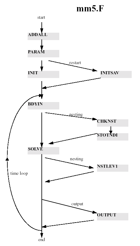
This is a brief, and not very thorough, description of the model's code. The main program is MM5 (filename is ./Run/mm5.F). This calls routines to initialize the pointer addresses (ADDALL), the model constants (PARAM), to restart (INITSAV) or initialize and read in (INIT) the model arrays, and to read in boundary conditions (BDYIN). It then executes the main time loop of the program. If there is no nest the time loop just has a call to SOLVE and occasional calls to OUTPUT. SOLVE is the routine that calls all the physics and dynamics routines and is responsible for all the model calculations. If there is a nest, there is a call to STOTNDI before SOLVE to define the initial nest boundary values by interpolation from the coarse mesh, and after SOLVE there is a call to a driver routine NSTLEV1. The main program is also responsible through CHKNST for initializing and ending nest.
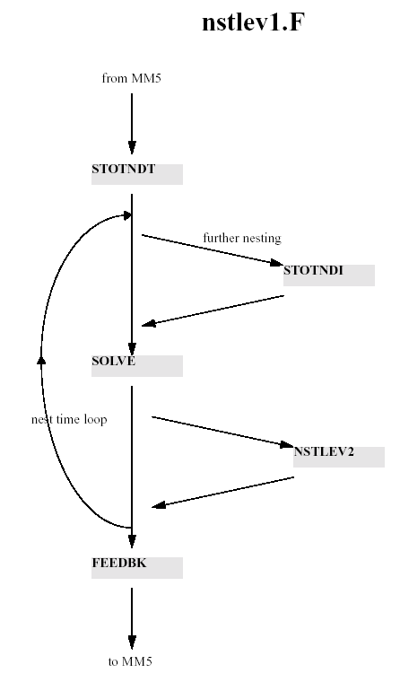
NSTLEV1 calls STOTNDT which calculates the nest boundary tendency based on that of the coarse mesh which is known after SOLVE has been called. It then executes three nested timesteps, which are one third of the coarse mesh's, in which it calls SOLVE for the nested domain, thus advancing that domain to the same time as the coarse mesh. It then calls FEEDBK to overwrite the coarse mesh values that coincide with nested grid-points. If there is a further nested level, NSTLEV1 will also call STOTNDI and NSTLEV2 for each subdomain at the next level.
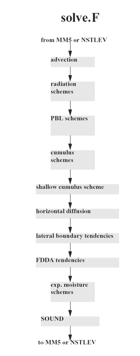
SOLVE is the main solver routine in which all the fields are advanced to the next time level. It does this by calling routines that calculate tendencies due to advection (VADV, HADV), diffusion (DIFFU, DIFFUT), PBL (e.g. HIRPBL), cumulus (e.g. CUPARA2), explicit moisture (e.g. EXMOISS), radiation (e.g. LWRAD, SWRAD), FDDA (NUDOB, NUDGD), boundary conditions (NUDGE), and dynamics (SOUND). In addition some tendencies are added within SOLVE itself, such as the adiabatic temperature term and the buoyancy and Coriolis momentum terms.
SOUND handles some terms using a short timestep. These terms, responsible for acoustic modes, are the pressure gradient terms in the momentum equations and the divergence term in the pressure tendency. Thus, only after SOUND are the momentum components and pressure updated while all the other prognostic variables are updated in SOLVE.
