E: 3DVAR

E.1.1 The Data Assimilation Problem

 

A data assimilation system combines all available information on the atmospheric state in a given time-window to produce an estimate of atmospheric conditions valid at a prescribed analysis time. Sources of information used to produce the analysis include observations, previous forecasts (the background or first-guess state), their respective errors and the laws of physics. The analysis can be used in a number of ways, including:

 

• Providing initial conditions for a numerical weather forecast (initialization).
• Studying climate through the merging of observations and numerical models (reanalysis).
• Assessing the impact of individual components of the existing observation network via Observation System Experiments (OSEs).
• Predicting the potential impact of proposed new components of a future observation network via Observation System Simulation Experiments (OSSEs).

 

The importance of accurate initial conditions to the success of an assimilation/forecast numerical weather prediction (NWP) system is well known. The relative importance of forecast errors due to errors in initial conditions compared to other sources of error such as physical parameterizations, boundary conditions and forecast dynamics depends on a number of factors e.g. resolution, domain, data density, orography as well as the forecast product of interest. However, judging from the current/future-planned resources (computational and human) of both operational and research communities being devoted to data assimilation, better initial conditions are increasingly considered vital for a whole range of NWP applications. Initial applications of the MM5 3DVAR system have focused on providing initial conditions from which to integrate MM5 forecasts. Future use of the system for regional climate modeling, OSEs and OSSEs is an exciting possibility.

 

E.1.2 Variational Data Assimilation

 

In recent years, much effort has been spent in the development of variational data assimilation systems to replace previously used schemes e.g. the Cressman (MM5), Newtonian nudging (FDDA -MM5), optimum interpolation (OI - NCEP, ECMWF, HIRLAM, NRL, etc.) and analysis correction (UKMO) algorithms. Practical considerations have led to a variety of alternative implementations of VAR systems.

 

The basic goal of the MM5 3DVAR system is to produce an "optimal" estimate of the true atmospheric state at analysis time through iterative solution of a prescribed cost-function (Ide et al. 1997)

 

(E.1)

 

The VAR problem can be summarized as the iterative solution of Eq. (E.1) to find the analysis state x that minimizes J(x). This solution represents the a posteriori maximum likelihood (minimum variance) estimate of the true state of the atmosphere given the two sources of a priori data: the background (previous forecast) x b and observations y o (Lorenc 1986). The fit to individual data points is weighted by estimates of their errors: B, E and F are the background, observation (instrumental) and representivity error covariance matrices respectively. Representivity error is an estimate of inaccuracies introduced in the observation operator H used to transform the gridded analysis x to observation space y=Hx for comparison against observations. This error will be resolution dependent and may also include a contribution from approximations (e.g. linearizations) in H.

 

The quadratic cost function given by Eq. (E.1) assumes that observation and background error covariances statistically are described using Gaussian probability density functions with zero mean error. Alternative cost functions maybe used which relax these assumptions (e.g. Dharssi et al. 1992). Eq. (E.1) additionally neglects correlations between observation and background errors.

 

The use of adjoint operations, which can be viewed as a multidimensional application of the chain-rule for partial differentiation, permits efficient calculation of the gradient of the cost-function. Modern minimization techniques (e.g. Quasi-Newton, preconditioned conjugate gradient) are used to efficiently combine cost function, gradient and the analysis information to produce the "optimal" analysis.

 

The theoretical problem of minimizing the cost function J(x) is equivalent to the previous-generation OI technique in the linear case. Despite this equivalence, previously developed operational 3/4DVAR systems e.g. NCEP (1992), ECMWF (1996/8), Meteo-France (1998/2000), UKMO (1999) have led to improved forecast scores relatively quickly after implementation through their more flexible design. Below are listed practical advantages of VAR systems over their predecessors.

 

• Observations can easily be assimilated directly without the need for prior retrieval. This results in a consistent treatment of all observations and, as the observation errors are less correlated (with each other and the background errors), practical simplifications to the analysis algorithm. 

• The VAR solution is found using all observations simultaneously, unlike the OI technique for which a data selection into artificial sub-domains is required. 

• Asynoptic data can be assimilated near its validity time. This is implicit to 4DVAR but can also be achieved using a "rapidly-updating" 3DVAR technique. 

• Balance (e.g. weak geostrophy, hydrostatic) constraints can be built into the preconditioning of the cost-function minimization. In 4DVAR, use is also made of the implicit balance of the forecast model.

Having expounded the advantages of variational data assimilation it is wise to also recognize its weaknesses. Although the variational analysis is frequently described as "optimal", this label is subject to a number of assumptions. Firstly, given both imperfect observations and prior (e.g. background) information as inputs to the assimilation system, the quality of the output analysis depends crucially on the accuracy of prescribed errors. Secondly, although the variational method allows for the inclusion of linearized dynamical/physical processes, in reality real errors in the NWP system may be highly nonlinear. This limits the usefulness of variational data assimilation in highly nonlinear regimes e.g. the convective scale or in the tropics. It is hoped that the 3DVAR system will be used in future studies to investigate these research topics.

 

In the development of variational data assimilation systems at the operational centers, 3DVAR has been seen as a necessary prerequisite to the ultimate goal of four-dimensional (e.g. 4DVAR/Kalman-filter-type) assimilation algorithms. Their initial concentration on 3DVAR has been partly motivated by a lack of computing resources (with the current exceptions of ECMWF and Meteo-France which now run 4DVAR operationally). Without the cut-off time restrictions of the weather centers, the research community has tended to bypass 3DVAR to concentrate on applications of 4DVAR to new/asynoptic data types e.g. Doppler radar.

 

 

E.2.1 Background Preprocessing

 

In cold-starting mode, standard MM5 preprocessing programs may be used to reformat and interpolate forecast fields from a variety of sources to the target MM5 domain. These packages are:

 

• TERRAIN - defines domain, orography, land use etc.
• PREGRID - reads background forecast in native format e.g. RUC, ETA, AVN, ECMWF etc.
• REGRIDDER - horizontally interpolates background to MM5 domain.
• INTERPF - vertically interpolates background field to MM5 sigma-height levels.

 

For further details on any of the above MM5 preprocessing packages, refer to the documentation on the MM5 web-page: http://www2.mmm.ucar.edu/mm5. In cycling mode, background processing is not required as the background field x b input to 3DVAR is already on the MM5 grid.

 

E.2.2 The Observation Preprocessor (3DVAR_OBSPROC)

 

The observation preprocessor provides the observations y o for ingest into 3DVAR. The program 3DVAR_OBSPROC has been specially written for use with the MM5 3DVAR system. It performs the following functions:

 

• Reads in observation file in decoder (MM5 LITTLE_R format).
• Reads in run-time parameters from a namelist file.
• Performs spatial and temporal checks to select only observations located within the target domain and within a specified time-window.
• Calculates heights for observations whose vertical coordinate is pressure.
• Merges duplicate observations (same location, place, type) and chooses observation nearest analysis time for stations with observations at several times.
• Estimates the error for each observation.
• Outputs observation file in ASCII 3DVAR format.

 

Further details may be found in Section 3 of the NCAR Technical Note (Barker et al. 2003).

 

E.2.3 Background Error Calculation

 

Background error covariance statistics are used in the 3DVAR cost-function to weight errors in features of the background field. The assimilation system will filter those background structures that have high error relative to more accurately known background features and observations. In reality, errors in the background field will be synoptically-dependent i.e. vary from day to day depending on the current weather situation. Current implementations of 3DVAR however, tend to use climatological background errors although research is ongoing into the specification and use of background "errors of the day".

 

The NMC-method (Parrish and Derber 1992) is a popular method for estimating climatological background error covariances. In this process, background errors are assumed to be well approximated by averaged forecast difference (e.g. month-long series of 24hr - 12hr forecasts valid at the same time) statistics:

 

(E.2)

 

where x t is the true atmospheric state and is the background error. The overbar denotes an average over time and/or space. Technical details of the NMC-method code developed in NCAR/MMM may be found in section 8 of the NCAR Technical Note (Barker et al. 2003). In the current MM5 3DVAR, the background errors are computed for a variety of resolutions and a seasonal dependence is introduced simply by using forecast difference statistics valid at different times of the year (e.g. winter, summer).

 

It is clear that the background errors should estimate errors in the analysis/forecast used as starting point for the 3DVAR minimization. In cold-starting mode, the background field originates from a different model (e.g. AVN, CWBGM). In contrast, a cycling application requires errors representative of a short-range forecast run from a previous 3DVAR analysis. Background errors will vary between each application and should ideally be tuned for each domain. This is time-consuming, but important, work. A recalculation of background error should be considered whenever the background field changes. Scenarios where this might occur include:

 

• Using an alternative source for the background field in cold-starting mode.
• The cold-starting background has been upgraded (e.g. change of resolution, additional observations used in a global analysis background).
• Change to MM5 configuration in a cycling run.

 

The initial period of a new cycling application must initially use background errors interpolated from another source of similar resolution/location. Once the new domain has been running for a period (e.g. 1 month) a better estimate of background error may be obtained. This is an iterative process - changing the background error used in 3DVAR will again modify background errors of the resulting short-range forecast used as background.

 

The calculation of background error covariances requires significant resources that are not always available. Given this limitation, and the fact that the background errors derived by the "NMC-method" are climatological estimates, approximations are inevitable. 3DVAR includes a number of namelist variables that allow some tuning of the background error files at run-time.

 

E.2.4 3DVAR System Overview

 

Although the 3DVAR code is completely new, the particular 3DVAR implementation described below is similar in basic design to that implemented operationally at the UK Meteorological Office in 1999 (Lorenc et al. 2000). In summary, the main features of the MM5 3DVAR system include:

 

• Incremental formulation of the model-space cost function given by Eq. (1) with the outer loop implemeted in considering the nonlineat effects of the observation operators and doing the `variational data quality control'.
• Quasi-Newton (QN) and Conjugate Gradient (CG) minimization algorithm.
• Analysis increments on unstaggered "Arakawa-A" grid. In the MM5 environment, the input background wind field is interpolated from the Arakawa-B grid of MM5. On output, the unstaggered analysis wind increments are interpolated to the MM5 B-grid.
• Analysis performed on the sigma-height levels of MM5.
• Jb preconditioning via a "control variable transform" U defined as B=UU T .
• Preconditioned control variables are chosen as streamfunction, velocity potential, unbalanced pressure and a choice between specific or relative humidity.
• Linearized mass-wind balance (including both geostrophic and cyclostrophic terms) used to define a balanced pressure.
• Climatological background error covariances estimated via the NMC-method of averaged forecast differences. Values are tuned by comparison with estimates derived from observation minus background differences (innovation vector) statistics.
• Representation of the horizontal component of background error via isotropic recursive filters. The vertical component is applied through projection onto climatologically averaged eigenvectors of vertical error (estimated via the NMC-method. Horizontal/vertical errors are non-separable (horizontal scales vary with vertical eigenvector).

 

Further details can be found in links from the NCAR/MMM 3DVAR web site (http://www2.mmm.ucar.edu/3dvar) including links to results of extended testing as well as the code (Fortran90 transformed to html using software designed in NCAR/MMM). The code itself contains a significant level of documentation.

 

E.2.5 Update Boundary Conditions

 

In order to run MM5 (or any other forecast model supported by the 3DVAR system) using the 3DVAR analysis as initial conditions, the lateral boundary conditions must first be modified to reflect differences between background forecast and analysis. This process is described in section 10 of the NCAR Technical Note (Barker et al. 2003).

 

 

E.3.1 Observation Preprocessor Tasks

 

The observation preprocessor performs the following functions:

 

1. Reads in observation file in decoder (LITTLE_R) format.

 

This format is that output by MM5 decoder routines and previously used in the preexisting MM5 LITTLE_R analysis package. This format was adopted as input to 3DVAR_OBSPROC in order to allow easy comparison of 3DVAR with LITTLE_R (which 3DVAR is intended to replace). A description of the LITTLE_R data format can be found at:

 

http://www2.mmm.ucar.edu/mm5/documents/MM5_tut_Web_notes/OA/OA.html

 

2. Reads in run-time parameters from a namelist file. An example is given below:

 

&record1

obs_gts_filename = '/mmmtmp/bresch/3dv/obs',

obs_err_filename = 'obserr.txt',

obs_gps_filename = 'NOGPS',

first_guess_file = '/mmmtmp/bresch/3dv/MMINPUT_DOMAIN2',

/

 

&record2

time_earlier = -90,

time_analysis = '2001-06-27_12:00:00',

time_later = 90,

/

 

&record3

max_number_of_obs = 58000,

fatal_if_exceed_max_obs = .TRUE.,

/

 

&record4

qc_test_vert_consistency = .TRUE.,

qc_test_convective_adj = .TRUE.,

qc_test_above_lid = .TRUE.,

remove_above_lid = .TRUE.,

Thining_SATOB = .FALSE.,

Thining_SSMI = .FALSE.,

/

 

&record5

print_gts_read = .TRUE.,

print_gpspw_read = .TRUE.,

print_recoverp = .TRUE.,

print_duplicate_loc = .TRUE.,

print_duplicate_time = .TRUE.,

print_recoverh = .TRUE.,

print_qc_vert = .TRUE.,

print_qc_conv = .TRUE.,

print_qc_lid = .TRUE.,

print_uncomplete = .TRUE.,

user_defined_area = .FALSE.,

/

 

&record6

x_left = 1.,

x_right = 100.,

y_bottom = 1.,

y_top = 100.,

/

 

3. Performs spatial and temporal checks to select only observations located within the target domain and within a specified time-window.

 

4. Calculates heights for observations whose vertical coordinate is pressure.

 

5. Merges duplicate observations (same location, place, type) and chooses observation nearest analysis time for stations with observations at several times.

 

6. Estimates the error for each observation. Values are input from the "obserr.txt" file containing observation errors at standard pressure levels for a number of different observation types. The errors tabulated in file "obserr.txt" originate from NCEP but have been modified at NCAR after comparisons against O-B data.

 

7. Outputs observation file in ASCII MM5 3DVAR format read for input to 3DVAR. An example header of the observation file is given below.

 

TOTAL = 8170, MISS. =-888888.,

SYNOP = 1432, METAR = 164, SHIP = 86, TEMP = 180, AMDAR = 0,

AIREP = 265, PILOT = 0, SATEM = 0, SATOB = 6043, GPSPW = 0,

SSMT1 = 0, SSMT2 = 0, TOVS = 0, OTHER = 0,

PHIC = 28.50, XLONC = 116.00, TRUE1 = 10.00, TRUE2 = 45.00,

TS0 = 275.00, TLP = 50.00, PTOP = 7000., PS0 =100000.,

IXC = 67, JXC = 81, IPROJ = 1, IDD = 1, MAXNES= 10,

NESTIX= 67, 67, 67, 67, 67, 67, 67, 67, 67, 67,

NESTJX= 81, 81, 81, 81, 81, 81, 81, 81, 81, 81,

NUMC = 1, 1, 1, 1, 1, 1, 1, 1, 1, 1,

DIS = 135.00, 0.00, 0.00, 0.00, 0.00, 0.00, 0.00, 0.00, 0.00, 0.00,

NESTI = 1, 1, 1, 1, 1, 1, 1, 1, 1, 1,

NESTJ = 1, 1, 1, 1, 1, 1, 1, 1, 1, 1,

INFO = PLATFORM, DATE, NAME, LEVELS, LATITUDE, LONGITUDE, ELEVATION, ID.

SRFC = SLP, PW (DATA,QC,ERROR).

EACH = PRES, SPEED, DIR, HEIGHT, TEMP, DEW PT, HUMID (DATA,QC,ERROR)*LEVELS.

INFO_FMT = (A12,1X,A19,1X,A40,1X,I6,3(F12.3,11X),6X,A5)

SRFC_FMT = (F12.3,I4,F7.2,F12.3,I4,F7.2)

EACH_FMT = (3(F12.3,I4,F7.2),11X,3(F12.3,I4,F7.2),11X,1(F12.3,I4,F7.2)))

........observations........

 

 

The header contains information on the number of observations for each type and the grid that has been used to select observations. The final three lines above define the format used to store particular observations which follow the header and which are subsequently read by 3DVAR. The observation preprocessor also has the capability to input observations in BUFR format. This latter format is not used in MM5 applications.

 

8. 3DVAR_OBSPROC outputs numerous diagnostics files that detail the quality control decisions taken and error estimates used.

 

E.3.2 Quality Control Flags used in 3DVAR_OBSPROC and 3DVAR

 

A variety of quality control checks are performed by the observation preprocessor. Quality control flags are set for all observations and output ready for input into 3DVAR. The following flags are currently used:

 

missing_data = -88, & ! Data is missing with the value of missing_r

outside_of_domain = -77, & ! Data outside horizontal domain

! or time window, data set to missing_r

wrong_direction = -15, & ! Wind vector direction <0 or> 360

! => direction set to missing_r

negative_spd = -14, & ! Wind vector norm is negative

! => norm set to missing_r

zero_spd = -13, & ! Wind vector norm is zero

! => norm set to missing_r

wrong_wind_data = -12, & ! Spike in wind profile

! =>direction and norm set to missing_r

zero_t_td = -11, & ! t or td = 0 => t or td, rh and qv

! are set to missing_r,

t_fail_supa_inver = -10, & ! superadiabatic temperature

!

wrong_t_sign = - 9, & ! Spike in Temperature profile

!

above_model_lid = - 8, & ! height above model lid

! => no action

far_below_model_surface = - 7, & ! height far below model surface

! => no action

below_model_surface = - 6, & ! height below model surface

! => no action

standard_atmosphere = - 5, & ! Missing h, p or t

! =>Datum interpolated from standard atm

from_background = - 4, & ! Missing h, p or t

! =>Datum interpolated from model

fails_error_max = - 3, & ! Datum Fails error max check

! => no action

fails_buddy_check = - 2, & ! Datum Fails buddy check

! => no action

no_buddies = - 1, & ! Datum has no buddies

! => no action

good_quality = 0, & ! OBS datum has good quality

!

convective_adjustment = 1, & ! convective adjustment check

! =>apply correction on t, td, rh and qv

surface_correction = 2, & ! Surface datum

! => apply correction on datum

Hydrostatic_recover = 3, & ! Height from hydrostatic assumption with

! the OBS data calibration

Reference_OBS_recover = 4, & ! Height from reference state with OBS

! data calibration

Other_check = 88 ! passed other quality check

 

The obervation preprocessor code can be downloaded from 3DVAR tutorial page by clicking Online 3DVAR tutorial from http://www2.mmm.ucar.edu/3dvar.

 

E.4.1 Overview

 

 

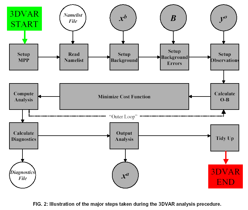
The top-level structure of 3DVAR is shown in Fig. 2. The 3DVAR runs under the WRF model framework to permit access to WRF MPP software, required for applications of 3DVAR on multiple processor platforms. In future, this arrangement will also allow easy access to other parts of the WRF system (e.g. I/O) from 3DVAR (and vice versa). The 3DVAR algorithm is called as a "mediation layer" subroutine from the WRF driver.

 

The following summarizes the role of each step in the 3DVAR algorithm:

• Setup MPP: Details of the run configuration are read in from a WRF namelist file. Tile, memory and domain dimension are calculated and stored.
  
• Read [3DVAR] Namelist: 3DVAR run-time options are read in from a namelist file. These options are described more fully in Appendix D of the NCAR Technical Note (Barker et al. 2003). The details can also be found from 3DVAR tutorial page.
  
• Setup Background: The background field x b is read in (MM5 format for MM5 applications, WRF format for WRF). Variables required by 3DVAR are stored in the xb Fortran90 derived data type (e.g. xb % u, xb % v etc.). Any additional fields present in the input file are ignored.
  
• Setup Background Errors: Components of the background error (eigenvectors, eigenvalues, lengthscales and balance regression coefficients) are read in (currently in MM5 format) and stored in the be derived data type (e.g. be % v1, be % reg_coeff etc.).
  
• Setup Observations: Observations y o and metadata (output from the observation preprocessor) are read (in either MM5 3DVAR ASCII or BUFR format) and stored in the ob derived data type (e.g. ob % synop % lat, ob % sonde % u, etc.). Basic quality control checks are again applied (e.g. domain checks) and an initial quality control flag is assigned.
  
• Calculate O-B: For valid data, the innovation vector y o - y b is calculated and stored in the iv derived data type (of similar design to the ob structure but including additional metadata). The transform y b = H(x b ) of the full-resolution background x b to observation space uses the nonlinear observation operator H. This transform involves both a change from model to observation variable and interpolation from grid points to the observation location. A "maximum error check" is applied to all values within the innovation vector iv which compares the O-B value against a maximum value defined as a multiple of the observation error for each observation. Various namelist parameters exist to tune QC checks as well as ones to choose which QC flags to ignore.
  
• Minimize Cost Function: The minimization of the 3DVAR cost function proceeds iteratively as described below. Diagnostic output includes cost function and gradient norm values for each iteration.
  
• Calculate Analysis: Having found the control variables that minimize the cost function, a final transform of the analysis increments to model (i.e. gridded u, v, T, p, q) space is performed. The increments are added to the background values to produce the analysis. Finally, checks are performed to ensure certain variables are within physically reasonable limits (e.g. relative humidity is greater than zero and less that 100%). The increments are adjusted if analysis values fall outside this range.
  
• Compute Diagnostics: Assimilation statistics (minimum, maximum, mean and root mean square) are calculated and output for study e.g. O-B, O-A statistics for each observation type, A-B (increment) statistics for each model variable. Output files are described in Appendix E of the NCAR Technical Note (Barker et al. 2003).
  
• Output Analysis: Both analysis and analysis increments are output.
  
• Tidy Up: Dynamically allocated memory is deallocated and summary run-time data output.
   

The "outer loop" seen in Fig. 2 permits the recalculation of the innovation vector using the analysis as an improved "background". The recalculation of O-B uses the full nonlinear observation operator H and hence provides a way if introducing nonlinearities into the analysis procedure. In addition, quality control checks based on maximum O-B values can be repeated. This equates to a crude "variational quality control" through the possibility that observation previously rejected due to too large an O-B value may be accepted in subsequent outer loops if the new O-B drops below the specified maximum value.

 

 

E.4.2 3DVAR Preconditioning Method

 

This subsection contains some of the mathematics behind the solution method chosen for the 3DVAR system. As stated above, the basic problem is to find the analysis state x a that minimizes a chosen cost function, here given by Eq. (1). For a model state x with n degrees of freedom, calculation of the background term J b of the cost function requires ~O(n 2 ) calculations. For a typical NWP model with n ~ 10 6 - 10 7 (number of grid-points times number of independent variables) direct solution is prohibitively expensive.

 

One practical solution to this problem is to perform a preconditioning via a control variable v transform defined by x' = Uv, where x' = x - x b . The transform U is chosen to approximately satisfy the relationship B=UU T . Using the incremental formulation (Courtier et al. 1994) and the control variable transform, eq. (1) may be rewritten

 

(E.3)

 

where y o' = y o - H(x b ) is the innovation vector and H is the linearization of the potentially nonlinear observation operator H used in the calculation of y o' . In this form, the background term is essentially diagonalized, reducing the number of calculations required from O(n 2 ) to O(n). In addition, the background error covariance matrix equals the identity matrix I in control variable space, hence preconditioning the minimization procedure.

 

The use of the incremental method has a number of advantages. Firstly, use of linear control variable transforms allows the straightforward use of adjoints in the calculation of the gradient of the cost function. Secondly, any imbalance introduced through the analysis procedure is limited to the (small) increments that are added to the balanced first guess. This generally leads to a more balanced analysis than that obtained using a technique in which the full-field analysis is constructed.

 

The transformation x' = Uv must be designed to ensure the validity of the B=UU T relationship. One goal is to transform to variables whose errors are largely uncorrelated with each other thus reducing B to block-diagonal form. In addition, each component of v is essentially scaled by the appropriate background error variance to allow an accurate penalization in the transformed J b cost function.

 

The 3DVAR control variable transform x' = Uv is in practice composed of a series of operations x' = U p U v U h v . The transformation always proceeds from control to model space (but is reversed in the adjoint code and the calculation of control variable background error statistics via the NMC-method). The individual operators represent in order the horizontal, vertical and change of physical variable transforms. In the MM5 3DVAR algorithm, the horizontal transform U h is performed using recursive filters to represent horizontal background error correlations. The vertical transform U v is applied via a projection from eigenvectors of a climatological estimate of the vertical component of background error onto model levels. Finally, the physical variable transformation U p converts control variables to model variables (e.g. u, v, T, p, q). Each stage of the control variable transform is discussed in the NCAR Technical Note (Barker et al. 2003)

 

E.4.3 3DVAR Source Code Organization

 

This section provides a brief tour around the 3DVAR code. Significant efforts have been made to make the code self-documenting, so this section should be seen as a prelude to looking at the code itself.

 

The use of Fortran90 has a number of advantages in designing a flexible, clear code. Firstly, the use of derived data types e.g. to store observations and their metadata significantly reduces the clutter that would be required in an equivalent Fortran77 code in which all components (e.g. station identifiers, location, quality control flags, errors, values etc.) would be separate entities. The entire observation structure can be represented as a single subroutine argument in which details are hidden. An extra advantage is that if a low level routine requires additional components of the data type to be written, then the calling tree above that routine stays the same.

 

The use of subroutine and variable names longer than the 31-character limit improves the readability of Fortran90 relative to Fortran77 code. Care must be taken in the use of some Fortran90 intrinsic procedures and dynamical allocation of memory. Experience has shown that, on certain platforms, use of these features may increase CPU relative to their Fortran77 counterparts.

 

 

 

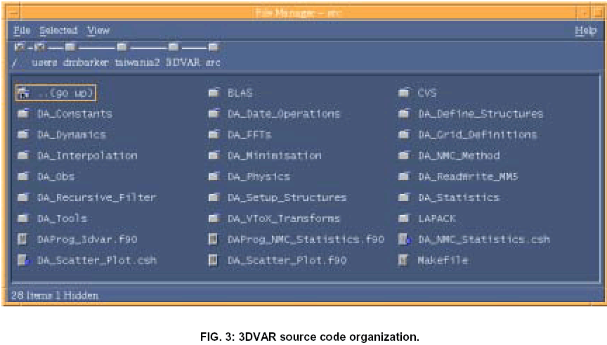
The 3DVAR source code is split into subdirectories containing logically distinct algorithms. Fig. 3 illustrates the setup for an earlier serial version of the code. As well as making the 3DVAR code easier to follow, the idea is to identify aspects that could be used, replaced or shared with code in the wider WRF framework in which 3DVAR resides e.g. general dynamics, physic and interpolation code.

 

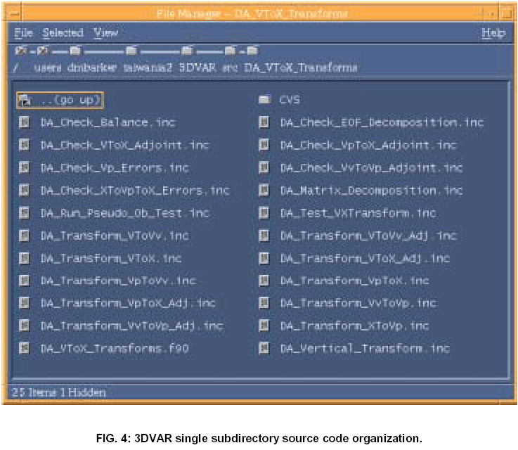
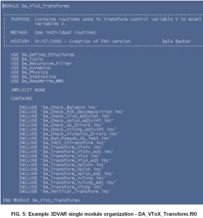
Each subdirectory within Fig. 3 is identified with a particular Fortran90 module file i.e. all the routines within the subdirectory are "Fortran90 INCLUDEd" in a single module file with the same name as the subdirectory (and the filetype .f90). Fig. 4 gives an example of the DA_VToX_Transforms subdirectory of Fig. 3. By convention, the module file in the DA_VToX_Transforms subdirectory shown in Fig. 4 is named DA_VToX_Transforms.f90 and CONTAINS all other (scientific) routines within the directory. The references within DA_VToX_Transforms.f90 to other subroutines within the DA_VToX_Transforms directory are seen in Fig. 5.  

 

  

Other reasons for adopting this code structure include the use of available automatic makefile generation scripts (which search .f90 files and routines specified in their INCLUDE lines). Also, experience has shown that this approach makes use of automatic Fortran->html tools much easier - common subdirectory, file and subroutine naming conventions are required to utilize this very useful facility.