
The goal of objective analysis in meteorological modeling is to improve meteorological analyses (the first guess ) on the mesoscale grid by incorporating information from observations. Traditionally, these observations have been "direct" observations of temperature, humidity, and wind from surface and radiosonde reports. As remote sensing techniques come of age, more and more "indirect" observations are available for researchers and operational modelers. Effective use of these indirect observations for objective analysis is not a trivial task. Methods commonly employed for indirect observations include three-dimensional or four-dimensional variational techniques ("3DVAR" and "4DVAR", respectively), which can be used for direct observations as well.
The MM5 system has long included packages for objective analysis of direct observations: the RAWINS program and the LITTLE_R program. A recent additon to the MM5 system is the 3DVAR package, which allows for variational assimilation of both direct observations and certain types of indirect observations. This chapter discusses the objective analysis program, LITTLE_R, which is perhaps best suited to new MM5 users. Some reference is made to the older RAWINS program (some details are available in Appendix F). Discussion of 3DVAR is reserved for Appendix E.
The analyses input to LITTLE_R and RAWINS as the first guess are usually fairly low-resolution analyses output from program REGRID. LITTLE_R and RAWINS may also use an MM5 forecast (through a back-end interpolation from sigma to pressure levels) as the first guess.
LITTLE_R and RAWINS capabilities include:
Users are strongly encouraged to use LITTLE_R for the objective analysis step. Most of what you'll need to do is done more easily in LITTLE_R than in RAWINS.
Input of observations is perhaps the greatest difference between LITTLE_R and RAWINS. RAWINS was developed around a specific set of data in a specific format. Incorporating data into RAWINS from unexpected sources or in different formats tends to be a challenge. LITTLE_R specifies it's own format for input (which has it's own challenges), but is better suited for users to adapt their own data.
RAWINS incorporates data from NCEP operational global surface and upper-air observations subsets as archived by the Data Support Section (DSS) at NCAR .
NMC Office Note 29 can be found in many places on the World Wide Web, including:
http://www.emc.ncep.noaa.gov/mmb/papers/keyser/on29.htm.
LITTLE_R reads observations provided by the user in formatted ASCII text files. The LITTLE_R tar file includes programs for converting the above NMC ON29 files into the LITTLE_R Observations Format. A user-contributed (i.e., unsupported) program is available on the MM5 ftp site for converting observations files from the GTS to LITTLE_R format. Users are responsible for converting other observations they may want to provide LITTLE_R into the LITTLE_R format. The details of this format are provided in section 6.12.
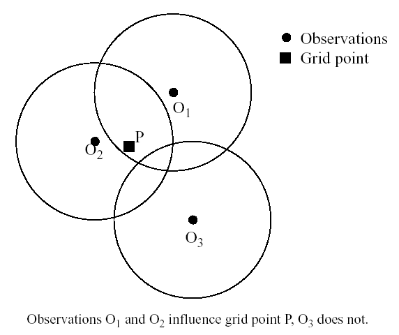
Three of the four objective analysis techniques used in LITTLE_R and RAWINS are based on the Cressman scheme, in which several successive scans nudge a first-guess field toward the neighboring observed values.
The standard Cressman scheme assigns to each observation a circular radius of influence R. The first-guess field at each gridpoint P is adjusted by taking into account all the observations which influence P.
The differences between the first-guess field and the observations are calculated, and a distance-weighted average of these difference values is added to the value of the first-guess at P. Once all gridpoints have been adjusted, the adjusted field is used as the first guess for another adjustment cycle. Subsequent passes each use a smaller radius of influence.
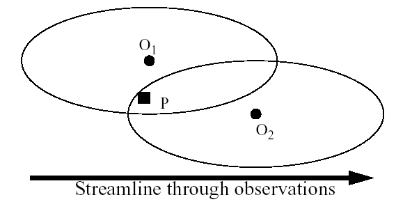
In analyses of wind and relative humidity (fields strongly deformed by the wind) at pressure levels, the circles from the standard Cressman scheme are elongated into ellipses oriented along the flow. The stronger the wind, the greater the eccentricity of the ellipses. This scheme reduces to the circular Cressman scheme under low-wind conditions.
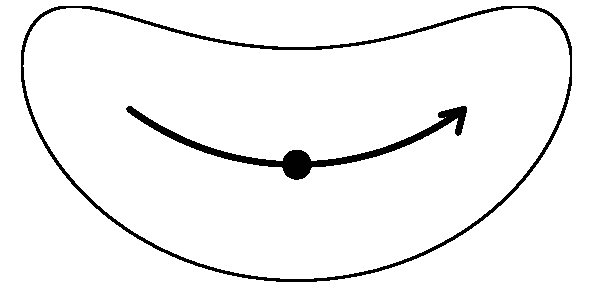
In analyses of wind and relative humidity at pressure levels, the circles from the standard Cressman scheme are elongated in the direction of the flow and curved along the streamlines. The result is a banana shape. This scheme reduces to the Ellipse scheme under straight-flow conditions, and the standard Cressman scheme under low-wind conditions.
The Multiquadric scheme uses hyperboloid radial basis functions to perform the objective analysis. Details of the multiquadric technique may be found in Nuss and Titley, 1994: "Use of multiquadric interpolation for meteorological objective analysis." Mon . Wea . Rev ., 122, 1611-1631. Use this scheme with caution, as it can produce some odd results in areas where only a few observations are available.
A critical component of LITTLE_R and RAWINS is the screening for bad observations. Many of these QC checks are done automatically in RAWINS (no user control), they are optional in LITTLE_R.
Most of these QC checks are done automatically in RAWINS (no user control), most are optional in LITTLE_R.
The ERRMAX quality-control check is optional (but highly recommended) in both LITTLE_R and RAWINS.
The Buddy check is optional (but highly recommended) in both LITTLE_R and RAWINS.
Input of additional observations, or modification of existing (and erroneous) observations, can be a useful tool at the objective analysis stage.
In LITTLE_R, additional observations are provided to the program the same way (in the same format) as standard observations. Indeed, additional observations must be in the same file as the rest of the observations. Existing (erroneous) observations can be modified easily, as the observations input format is ASCII text. Identifying an observation report as "bogus" simply means that it is assumed to be good data -- no quality control is performed for that report.
In RAWINS, the methods of adding or modifying observations are rather difficult to work with, requiring additional files with cryptic conventions. All observations provided through these files are assumed to be "good"; no quality control is performed on these observations. Don't try this unless it's absolutely necessary, and you're the patient sort. However, some people actually manage to use these procedures successfully. See notes on NBOGUS, KBOGUS, NSELIM in Appendix F.
The surface FDDA option creates additional analysis files for the surface only, usually with a smaller time interval between analyses (i.e., more frequently) than the full upper-air analyses. The purpose of these surface analysis files is for later use in MM5 with the surface analysis nudging option. This capability is turned on by setting the namelist option F4D = .TRUE., and selecting the time inteval in seconds for the surface analyses with option INTF4D.
A separate set of observations files is needed for the surface FDDA option in LITTLE_R. These files must be listed by the namelist record2 option sfc_obs_filename. A separate observations file must be supplied for each analysis time from the start date to the end date at time interval INTF4D.
The LAGTEM option controls how the first-guess field is created for surface analysis files. Typically, the surface and upper-air first-guess is available at twelve-hour intervals (00 Z and 12 Z), while the surface analysis interval may be set to 3 hours (10800 seconds). So at 00 Z and 12 Z, the available surface first-guess is used. If LAGTEM is set to .FALSE., the surface first-guess at other times will be temporally interpolated from the first-guess at 00 Z and 12 Z. If LAGTEM is set to .TRUE., the surface first guess at other times is the objective analysis from the previous time.
LITTLE_R and RAWINS have the capability to perform the objective analysis on a nest. This is done manually with a separate LITTLE_R or RAWINS process, performed on REGRID files for the particular nest. Often, however, such a step is unnecessary; it complicates matters for the user and may introduce errors into the forecast. At other times, extra information available to the user, or extra detail that objective analysis may provide on a nest, makes objective analysis on a nest a good option.
The main reason to do objective analysis on a nest is if you have observations available with horizontal resolution somewhat greater than the resolution of your coarse domain. There may also be circumstances in which the representation of terrain on a nest allows for better use of surface observations (i.e., the model terrain better matches the real terrain elevation of the observation).
The main problem introduced by doing objective analysis on a nest is inconsistency in initial conditions between the coarse domain and the nest. Observations that fall just outside a nest will be used in the analysis of the coarse domain, but discarded in the analysis of the nest. With different observations used right at a nest boundary, one can get very different analyses.
The source code is available via anonymous ftp, at
ftp://ftp.ucar.edu/mesouser/MM5V3/LITTLE_R.TAR.gz
Download this file to your local machine,
uncompress it, and untar it:
gzip -cd LITTLE_R.TAR.gz
tar -xvf LITTLE_R.TAR
You should now have a directory called LITTLE_R. Change to that directory:
The LITTLE_R executable is generated through the Make utility.
For a variety of common platforms and architectures, the Makefile is already
set up to build the executable. Simply type:
If your system is a little unusual, you may find yourself having to edit options in the Makefile.
For the tutorial exercises, there are prepared observations files for you to use. See the notes on the assignment.
A program is available for users with access to NCAR's computers to download archived observations and reformat them into the LITTLE_R Observations Format. See the information about the "fetch.deck" program, in section 6.14
A program is also available for reformatting observations from the GTS stream.
For other sources of data, the user is responsible for putting data into the LITTLE_R Observations Format. Hence the detailed discussion of the observations format in Section 6.12
In general, there are two overall strategies for organizing observations into observations files. The easiest strategy is to simply put all observations into a single file. The second strategy, which saves some processing time by LITTLE_R, is to sort observations into separate files by time.
For details about the namelist, see section 6.13. The most critical information you'll be changing most often are the start date, end date, and file names. Pay particularly careful attention to the file name settings. Mistakes in observations file names can go unnoticed because LITTLE_R will happily process the wrong files, and if there are no data in the (wrongly-specified) file for a particular time, LITTLE_R will happily provide you with an analysis of no observations.
Run the program by invoking the
command:
The ">! print.out" part of that command simply redirects printout into a file called "print.out".
Examine the "print.out" file for error messages or warning messages. The program should have created the file called "LITTLE_R_DOMAIN<#>", according to the domain number. Additional output files containing information about observations found and used and discarded will probably be created, as well.
Important things to check include the number of observations found for your objective analysis, and the number of observations used at various levels. This can alert you to possible problems in specifying observations files or time intervals. This information is included in the printout file.
You may also want to experiment with a couple of simple plot utility programs, discussed below.
There are a number of additional output files which you might find useful. These are discussed below.
The LITTLE_R program generates several ASCII text files to detail the actions taken on observations through a time cycle of the program (sorting, error checking, quality control flags, vertical interpolation). In support of users wishing to plot the observations used for each variable (at each level, at each time), a file is created with this information. Primarily, the ASCII text files are for consumption by the developers for diagnostic purposes. The main output of the LITTLE_R program is the gridded, pressure-level data set to be passed to the INTERPF program (file LITTLE_R_DOMAIN<#>).
In each of the files listed below, the text "_YYYY-MM-DD_HH:mm:ss.tttt" allows each time period that is processed by LITTLE_R to output a separate file. The only unusual information in the date string is the final four letters "tttt" which is the decimal time to ten thousandths (!) of a second. The bracketed "[sfc_fdda_]" indicates that the surface FDDA option of LITTLE_R creates the same set of files with the string "sfc_fdda_" inserted.
The final analysis file at surface and pressure levels. Generating this file is the primary goal of running LITTLE_R.
Use of the surface FDDA option in LITTLE_R creates a file called "SFCFDDA_DOMAIN<#>". This file contains the surface analyses at INTF4D intervals, analyses of T, u, v, RH, qv, psfc, pmsl, and a count of observations within 250 km of each grid point.
This file contains a listing of all of the observations available for use by the LITTLE_R program. The observations have been sorted and the duplicates have been removed. Observations outside of the analysis region have been removed. Observations with no information have been removed. All reports for each separate location (different levels but at the same time) have been combined to form a single report. Interspersed with the output data are lines to separate each report. This file contains reports discarded for QC reasons.
This file contains a listing of all of the observations available for use by the LITTLE_R program. The observations have been sorted and the duplicates have been removed. Observations outside of the analysis region have been removed. Observations with no information have been removed. All reports for each separate location (different levels but at the same time) have been combined to form a single report. Data which has had the "discard" flag internally set (data which will not be sent to the quality control or objective analysis portions of the code) are not listed in this output. No additional lines are introduced to the output, allowing this file to be reused as an observation input file.
This file only contains a listing of the discarded reports. This is a good place to begin to search to determine why an observation didn't make it into the analysis. This file has additional lines interspersed within the output to separate each report.
The information contained in the qc_out file is similar to the useful_out. The data has gone through a more expensive test to determine if the report is within the analysis region, and the data have been given various quality control flags. Unless a blatant error in the data is detected (such as a negative sea-level pressure), the observation data are not tyically modified, but only assigned quality control flags. Any data failing the error maximum or buddy check tests are not used in the objective analysis.
This file lists data by variable and by level, where each observation that has gone into the objective analysis is grouped with all of the associated observations for plotting or some other diagnostic purpose. The first line of this file is the necessary FORTRAN format required to input the data. There are titles over the data columns to aid in the information identification. Below are a few lines from a typical file.
( 3x,a8,3x,i6,3x,i5,3x,a8,3x,2(g13.6,3x),2(f7.2,3x),i7 )
Number of Observations 00001214
Variable Press Obs Station Obs Obs-1st X Y QC
Name Level Number ID Value Guess Location Location Value
U 1001 1 CYYT 6.39806 4.67690 161.51 122.96 0
U 1001 2 CWRA 2.04794 0.891641 162.04 120.03 0
U 1001 3 CWVA 1.30433 -1.80660 159.54 125.52 0
U 1001 4 CWAR 1.20569 1.07567 159.53 121.07 0
U 1001 5 CYQX 0.470500 -2.10306 156.58 125.17 0
U 1001 6 CWDO 0.789376 -3.03728 155.34 127.02 0
The LITTLE_R package provides two utility programs for plotting observations. These programs are called "plot_soundings"and "plot_levels". These optional programs use NCAR Graphics, and are built automatically if the PROGS option in the top-level Makefile is set to $(I_HAVE_NCARG). Both programs prompt the user for additional input options.
Program plot_soundings plots soundings. This program generates soundings from either the quality-controlled ("qc_out_yyyy-mm-dd_hh:mm:ss:ffff") or the non-quality-controlled ("useful_out_yyyy-mm-dd_hh:mm:ss:ffff") upper air data. Only data that are on the requested analysis levels are processed. The program asks the user for an input filename, and creates the file "soundings.cgm".
Program plot_level creates station plots for each analysis level. These plots contain both observations that have passed all QC tests and observations that have failed the QC tests. Observations that have failed the QC tests are plotted in various colors according to which test was failed. The program prompts the user for a date of the form yyyymmddhh, and plots the observations from file "plotobs_out_yyyy-mm-dd_hh:00:00:00.0000". The program creates the file "levels.cgm".
To make the best use of the LITTLE_R program, it is important for users to understand the LITTLE_R Observations Format.
Observations are conceptually organized in terms of reports. A report consists of a single observation or set of observations associated with a single latitude/longitude coordinate.
Each report in the LITTLE_R Observations Format consists of at least four records:
The report header
record is a 600-character long record (don't worry, much of it is unused
and needs only dummy values) which contains certain information about the
station and the report as a whole: location, station id, station type, station
elevation, etc. The report header record is described fully in the following
table. Shaded items in the table are unused:
|
Number of errors encountered during the decoding of this observation |
||
|
Number of warnings encountered during decoding of this observation. |
||
Following the report header record
are the data records . These data records contain
the observations of pressure, height, temperature, dewpoint, wind speed, and
wind direction. There are a number of other fields in the data record that
are not used on input. Each data record contains data for a single level of
the report. For report types which have multiple levels (e.g., upper-air station
sounding reports), each pressure or height level has its own data record.
For report types with a single level (such as surface station reports or a
satellite wind observation), the report will have a single data record. The
data record contents and format are summarized in the following table
The end data record is simply a data record with pressure and height fields both set to -777777.
After all the data records and the
end data record, an end report record must appear.
The end report record is simply three integers which really aren't all that
important.
|
Number of errors encountered during the decoding of the report |
||
|
Number of warnings encountered during the decoding the report |
In the observations files, most of the meteorological data fields also have space for an additional integer quality-control flag. The quality control values are of the form 2n, where n takes on positive integer values. This allows the various quality control flags to be additive yet permits the decomposition of the total sum into constituent components. Following are the current quality control flags that are applied to observations.
pressure interpolated from first-guess height = 2 ** 1 = 2
temperature and dew point both = 0 = 2 ** 4 = 16
wind speed and direction both = 0 = 2 ** 5 = 32
wind speed negative = 2 ** 6 = 64
wind direction < 0 or > 360 = 2 ** 7 = 128
level vertically interpolated = 2 ** 8 = 256
value vertically extrapolated from single level = 2 ** 9 = 512
sign of temperature reversed = 2 ** 10 = 1024
superadiabatic level detected = 2 ** 11 = 2048
vertical spike in wind speed or direction = 2 ** 12 = 4096
convective adjustment applied to temperature field = 2 ** 13 = 8192
no neighboring observations for buddy check = 2 ** 14 = 16384
---------------------------------------------------------------------------
fails error maximum test = 2 ** 15 = 32768
fails buddy test = 2 ** 16 = 65536
observation outside of domain detected by QC = 2 ** 17 = 131072
The LITTLE_R namelist file is called "namelist.input", and must be in the directory from which LITTLE_R is run. The namelist consists of nine namelist records, named "record1" through "record9", each having a loosely related area of content. Each namelist record, which extends over several lines in the namelist.input file, begins with "&record<#>" (where <#> is the namelist record number) and ends with a slash "/".
The data in namelist record1 define the analysis times to process:
&record1
start_year = 1990
start_month = 03
start_day = 13
start_hour = 00
end_year = 1990
end_month = 03
end_day = 14
end_hour = 00
interval = 21600
/
The data in record2 define the names of the input files:
&record2
fg_filename = '../data/REGRID_DOMAIN1'
obs_filename = '../data/obs1300'
obs_filename = '../data/obs1306'
obs_filename = '../data/obs1312'
sfc_obs_filename = '../data/obs1300'
sfc_obs_filename = '../data/obs1303'
sfc_obs_filename = '../data/obs1306'
sfc_obs_filename = '../data/obs1309'
sfc_obs_filename = '../data/obs1312'
/
The obs_filename and sfc_obs_filename settings can get confusing, and deserve some additional explanation. Use of these files is related to the times and time interval set in namelist record1, and to the F4D options set in namelist record8. The obs_filename files are used for the analyses for the full 3D dataset, both at upper-air and the surface. The obs_filename files should contain all observations, upper-air and surface, to be used for a particular analysis at a particular time. The sfc_obs_filename is used only when F4D=.TRUE., that is, if surface analyses are being created for surface FDDA nudging. The sfc_obs_filenames may be the same files as obs_filenames, and they should probably contain both surface and upper-air observations. The designation "sfc_obs_filename" is not intended to indicate that the observations in the file are at the surface, but rather that the file is used only for a surface analysis prepared for surface FDDA nudging.
There must be an obs_filename listed for each time period for which an objective analysis is desired. Time periods are processed sequentially from the starting date to the ending date by the time interval, all specified in namelist record1. For the first time period, the file named first in obs_filename is used. For the second time period, the file named second in obs_filename is used. This pattern is repeated until all files listed in obs_filename have been used. dor Subsequent time periods (if any), the first guess is simply passed to the output file without objective analysis.
If the F4D option is selected, the files listed in sfc_obs_filename are similarly processed for surface analyses, this time with the time interval as specified by INTF4D.
The data in the record3 concern space allocated within the program for observations. These are values that should not frequently need to be modified:
&record3
max_number_of_obs = 10000
fatal_if_exceed_max_obs = .TRUE.
/
|
T/F flag allows the user to decide the severity of not having enough space to store all of the available observations |
The data in record4 set the quality control options. There are four specific tests that may be activated by the user:
&record4
qc_test_error_max = .TRUE.
qc_test_buddy = .TRUE.
qc_test_vert_consistency = .FALSE.
qc_test_convective_adj = .FALSE.
max_error_t = 8
max_error_uv = 10
max_error_z = 16
max_error_rh = 40
max_error_p = 400
max_buddy_t = 10
max_buddy_uv = 12
max_buddy_z = 16
max_buddy_rh = 40
max_buddy_p = 400
buddy_weight = 1.0
max_p_extend_t = 1300
max_p_extend_w = 1300
/
For the error maximum tests, there is a threshold for each variable. These values are scaled for time of day, surface characteristics and vertical level.
|
maximum allowable horizontal wind component difference (m/s) |
||
For the buddy check test, there is a threshold for each variable. These values are similar to standard deviations.
|
maximum allowable horizontal wind component difference (m/s) |
||
For satellite and aircraft observations, data are often horizontally spaced with only a single vertical level. The following two entries describe how far the user assumes that the data are valid in pressure space.
|
pressure difference (Pa) through which a single temperature report may be extended |
||
|
pressure difference (Pa) through which a single wind report may be extended |
The data in record5 control the enormous amount of print-out which may be produced by the LITTLE_R program. These values are all logical flags, where TRUE will generate output and FALSE will turn off output.
&record5
print_obs_files = .TRUE.
print_found_obs = .FALSE.
print_header = .FALSE.
print_analysis = .FALSE.
print_qc_vert = .FALSE.
print_qc_dry = .FALSE.
print_error_max = .FALSE.
print_buddy = .FALSE.
print_oa = .FALSE.
/
The data in record7 concerns the use of the first-guess fields, and surface FDDA analysis options. Always use the first guess.
&record7
use_first_guess = .TRUE.
f4d = .TRUE.
intf4d = 10800
lagtem = .FALSE.
/
The data in record8 concern the smoothing of the data after the objective analysis. The differences (observation minus first-guess) of the analyzed fields are smoothed, not the full fields:
&record8
smooth_type = 1
smooth_sfc_wind = 1
smooth_sfc_temp = 0
smooth_sfc_rh = 0
smooth_sfc_slp = 0
smooth_upper_wind = 0
smooth_upper_temp = 0
smooth_upper_rh = 0
/
|
1 = five point stencil of 1-2-1 smoothing; 2 = smoother-desmoother |
||
The data in record9 concern the objective analysis options. There is no user control to select the various Cressman extensions for the radius of influence (circular, elliptical or banana). If the Cressman option is selected, ellipse or banana extensions will be applied as the wind conditions warrant.
&record9
oa_type = 'MQD'
mqd_minimum_num_obs = 50
mqd_maximum_num_obs = 1000
radius_influence = 12
oa_min_switch = .TRUE.
oa_max_switch = .TRUE.
/
An IBM job deck is provided to allow users with NCAR IBM access to use the traditional observations archives available to MM5 users from the NCAR Mass Storage System. It is located in the LITTLE_R/util directory, and called "fetch.deck.ibm". This job script retrieves the data from the archives for a requested time period, converts it to the LITTLE_R Observations Format, and stores these reformatted files on the Mass Storage System for the user to retrieve. The critical portion of the script is printed below:
# **********************************************
# ****** fetch interactive/batch C shell *****
# ******* NCAR IBM's only
******
# ******* f90
only ******
# **********************************************
#
# This shell fetches ADP data from the NCAR MSS system and
# converts it into a format suitable for the little_r
# program. The data are stored on the NCAR MSS.
#
# Three types of data files are created:
# obs:DATE : Upper-air and surface data used as
# input to little_R
# surface_obs_r:DATE : Surface data needed for FDDA in little_r
# (if no FDDA will be done, these are not
# needed, since they are also contained
# in obs:DATE)
# upper-air_obs_r:DATE : Upper-air data (this file is contained
# in obs:DATE file, and is not needed for
# input to little_r)
#
# This should be the user's case or experiment (used in MSS name).
# This is where the data will be stored on the MSS.
set ExpName = MM5V3/TEST # MSS path name for output
set RetPd = 365 # MSS retention period in days
# The only user inputs to the fetch program are the beginning
# and ending dates of the observations, and a bounding box for the
# observation search. These dates are given in YYYYMMDDHH. The
# ADP data are global, and include the surface observations and
# upper-air soundings. A restrictive bounding box (where
# possible) reduces the cost substantially.
#
# Note: No observational data are available prior to 1973, and
# no or limited surface observations are available
# prior to 1976.
set starting_date = 1993031300
set ending_date = 1993031400
set lon_e = 180
set lon_w = -180
set lat_s = -90
set lat_n = 90
#########################################################
######### #########
######### END OF USER MODIFICATIONS #########
######### #########
#########################################################