Welcome to the MPAS-JEDI tutorial practice guide

In order to build MPAS-JEDI and its dependencies, it is recommended to access source code from mpas-bundle. We will use the 'release/4.0.1' branch from mpas-bundle-4.0.1:

$ cd /glade/derecho/scratch/$USER/mpas_jedi_tutorial
$ mkdir mpas_bundle_v4
$ cd mpas_bundle_v4
$ git clone -b release/4.0.1 https://github.com/JCSDA/mpas-bundle code

The git command will clone the mpas-bundle repository from github to a local directory 'code' , then make the 'release/4.0.1' branch as the active branch. The output to the terminal should look as following:

Cloning into 'code'...
remote: Enumerating objects: 993, done.
remote: Counting objects: 100% (323/323), done.
remote: Compressing objects: 100% (135/135), done.
remote: Total 993 (delta 270), reused 193 (delta 188), pack-reused 670 (from 2)
Receiving objects: 100% (993/993), 272.94 KiB | 1.98 MiB/s, done.
Resolving deltas: 100% (627/627), done.

Note that the mpas-bundle repository does not contain actual source code. Instead, the CMakeLists.txt file under code includes the github repositories's branch/tag information needed to build MPAS-JEDI. We now create a 'build' folder and load the spack-stack environment pre-built using the GNU compiler:

$ source ./code/env-setup/gnu-derecho.sh
$ module list

The output to the module list in the terminal should look like the following (49 modules!!!). These packages are from pre-installed spack-stack-1.9.3.

Currently Loaded Modules:
  1) ecflow/5.8.4                 18) python-venv/1.0        35) snappy/1.2.1
  2) mysql/8.0.33                 19) py-setuptools/69.2.0   36) zstd/1.5.6
  3) stack-gcc/12.4.0             20) py-pycodestyle/2.11.0  37) c-blosc/1.21.5
  4) craype/2.7.31                21) boost/1.84.0           38) hdf5/1.14.3
  5) ncarenv/24.12           (S)  22) eigen/3.4.0            39) netcdf-c/4.9.2
  6) gcc/12.4.0                   23) openblas/0.3.24        40) netcdf-cxx4/4.3.1
  7) libfabric/1.15.2.0           24) eckit/1.28.3           41) netcdf-fortran/4.6.1
  8) cray-mpich/8.1.29            25) fftw/3.3.10            42) parallel-netcdf/1.12.3
  9) stack-cray-mpich/8.1.29      26) fckit/0.13.2           43) parallelio/2.6.2
 10) glibc/2.38                   27) fiat/1.4.1             44) gsl-lite/0.37.0
 11) tar/1.34                     28) ectrans/1.5.0          45) nccmp/1.9.0.1
 12) gettext/0.22.5               29) qhull/2020.2           46) udunits/2.2.28
 13) zlib/1.2.11                  30) atlas/0.40.0           47) py-numpy/1.26.4
 14) sqlite/3.46.0                31) nghttp2/1.63.0         48) bufr/12.1.0
 15) util-linux-uuid/2.40.2       32) curl/8.10.1            49) py-pybind11/2.13.5
 16) python/3.11.7                33) cmake/3.27.9
 17) stack-python/3.11.7          34) ecbuild/3.7.2

  Where:
   S:  Module is Sticky, requires --force to unload or purge

Now we are ready to 'fetch' actual source code from github repositories through cmake.

MPAS-JEDI uses cmake to automatically fetch the code from various github repositories, listed in CMakeLists.txt under ~code. Now type the command below under the build directory:

$ git lfs install
$ mkdir build
$ cd build
$ cmake ../code

The ioda-converters package is not built by default. To build the package, enable the BUILD_IODA_CONVERTERS option. Note that this will increase both the CMake configuration and compilation times.

$ cmake -DBUILD_IODA_CONVERTERS=ON ../code

After it completes (may take 15-20 min depending on network connection), you will see the actual source code of various repositories (e.g., oops, vader, saber, ufo, ioda, crtm, mpas-jedi, and MPAS) is now under the code directory. Meanwhile, Makefile files to build executables are generated under the build directory. Now it is ready to compile MPAS-JEDI under 'build' using the standard make. However, it is NOT recommended to compile the code on the login node. Instead, better compiling code using a compute node with an interactive job by issuing the command below:

$ qsub -A ummm0016 -N build-bundle -q tutorial -l job_priority=premium -l walltime=03:00:00 -l select=1:ncpus=128:mem=235GB -I

This requests an interactive job to the 'tutorial' queue, with a job name 'build-bundle', 3 hours walltime of a compute node with 128 cores, the 'premium' priority and an account number 'UMMM0016'.

Note that the interactive job does not have the spack-stack environment loaded, so you have to reload the spack-stack environment (under ~build), and then compiling code with the parallel make using 32 cores:

$ source ../code/env-setup/gnu-derecho.sh
$ make -j32

This could take ~10 min. Using more cores for build could speed up a bit, but will not help too much from our experience. Also note that the reason we do the cmake step (will clone various github repositories) on the login node instead of a compute node is that the derecho's compute nodes have a much slower internet connection.

Once we reach 100% of the compilation, many executables will be generated under ~build/bin. mpas model and mpas-jedi DA related executables are:

$ ls bin/mpas*
bin/mpas_atmosphere                      bin/mpasjedi_gen_ens_pert_B.x
bin/mpas_atmosphere_build_tables         bin/mpasjedi_hofx3d.x
bin/mpas_init_atmosphere                 bin/mpasjedi_hofx.x
bin/mpasjedi_convertstate.x              bin/mpasjedi_process_perts.x
bin/mpasjedi_converttostructuredgrid.x   bin/mpasjedi_rtpp.x
bin/mpasjedi_eda.x                       bin/mpasjedi_saca.x
bin/mpasjedi_enkf.x                      bin/mpasjedi_variational.x
bin/mpasjedi_enshofx.x                   bin/mpas_namelist_gen
bin/mpasjedi_ens_mean_variance.x         bin/mpas_parse_atmosphere
bin/mpasjedi_error_covariance_toolbox.x  bin/mpas_parse_init_atmosphere
bin/mpasjedi_forecast.x                  bin/mpas_streams_gen

The last step is to ensure that the code was compiled properly by running the MPAS-JEDI ctests, with two lines of simple command:

$ export LD_LIBRARY_PATH=/glade/derecho/scratch/${USER}/mpas_jedi_tutorial/mpas_bundle_v4/build/lib:$LD_LIBRARY_PATH
$ cd mpas-jedi
$ ctest

At the moment the tests are running (take ~5 min to finish), it indicates if it passes or fails. At the end, a summary is provided with a percentage of the tests that passed, failed and the processing times.

The output to the terminal should look as following:

......
100% tests passed, 0 tests failed out of 62
 
Label Time Summary:               
ci_oneapi_disable    =   5.68 sec*proc (1 test)
executable           =  44.25 sec*proc (12 tests)
mpasjedi             = 296.06 sec*proc (62 tests)
mpi                  = 294.14 sec*proc (61 tests)
script               = 251.80 sec*proc (50 tests)
tier2                = 122.04 sec*proc (15 tests)
   
Total Test time (real) = 296.22 sec

To determine if a test passes or fails, a comparison of the test log and reference file is done internally taking as reference a tolerance value. This tolerance is specified via YAML file. These files can be found under mpas-jedi/test/testoutput in the build folder:

3denvar_amsua_allsky.ref                   4denvar_VarBC_nonpar.run                forecast.ref
3denvar_amsua_allsky.run                   4denvar_VarBC_nonpar.run.ref            forecast.run
3denvar_amsua_allsky.run.ref               4denvar_VarBC.ref                       forecast.run.ref
3denvar_amsua_bc.ref                       4denvar_VarBC.run                       gen_ens_pert_B.ref
3denvar_amsua_bc.run                       4denvar_VarBC.run.ref                   gen_ens_pert_B.run
3denvar_amsua_bc.run.ref                   4dfgat_cda.ref                          gen_ens_pert_B.run.ref
3denvar_bumploc.ref                        4dfgat_cda.run                          hofx3d_nbam.ref
3denvar_bumploc.run                        4dfgat_cda.run.ref                      hofx3d_nbam.run
3denvar_bumploc.run.ref                    4dfgat.ref                              hofx3d_nbam.run.ref
3denvar_multi_resolution.ref               4dfgat.run                              hofx3d.ref
3denvar_multi_resolution_regional.ref      4dfgat.run.ref                          hofx3d_ropp.ref
3denvar_multi_resolution_regional.run      4dhybrid_bumpcov_bumploc.ref            hofx3d_rttovcpp.ref
3denvar_multi_resolution_regional.run.ref  4dhybrid_bumpcov_bumploc.run            hofx3d.run
3denvar_multi_resolution.run               4dhybrid_bumpcov_bumploc.run.ref        hofx3d.run.ref
3denvar_multi_resolution.run.ref           convertstate.ref                        hofx4d_pseudo.ref
3dfgat_cda.ref                             convertstate.run                        hofx4d_pseudo.run
3dfgat_cda.run                             convertstate.run.ref                    hofx4d_pseudo.run.ref
3dfgat_cda.run.ref                         converttostructuredgrid_latlon.ref      hofx4d.ref
3dfgat_pseudo.ref                          converttostructuredgrid_latlon.run      hofx4d.run
3dfgat_pseudo.run                          converttostructuredgrid_latlon.run.ref  hofx4d.run.ref
3dfgat_pseudo.run.ref                      dirac_bumpcov.ref                       letkf_3dloc.ref
3dfgat.ref                                 dirac_bumpcov.run                       letkf_3dloc.run
3dfgat.run                                 dirac_bumpcov.run.ref                   letkf_3dloc.run.ref
3dfgat.run.ref                             dirac_bumploc.ref                       lgetkf_height_vloc.ref
3dhybrid_bumpcov_bumploc.ref               dirac_bumploc.run                       lgetkf_height_vloc.run
3dhybrid_bumpcov_bumploc.run               dirac_bumploc.run.ref                   lgetkf_height_vloc.run.ref
3dhybrid_bumpcov_bumploc.run.ref           dirac_diffusion_duplicated.ref          lgetkf.ref
3dvar_bumpcov_nbam.ref                     dirac_diffusion_duplicated.run          lgetkf.run
3dvar_bumpcov_nbam.run                     dirac_diffusion_duplicated.run.ref      lgetkf.run.ref
3dvar_bumpcov_nbam.run.ref                 dirac_diffusion_univariate.ref          parameters_bumpcov.ref
3dvar_bumpcov.ref                          dirac_diffusion_univariate.run          parameters_bumpcov.run
3dvar_bumpcov_ropp.ref                     dirac_diffusion_univariate.run.ref      parameters_bumpcov.run.ref
3dvar_bumpcov_rttovcpp.ref                 dirac_noloc.ref                         parameters_bumploc.ref
3dvar_bumpcov.run                          dirac_noloc.run                         parameters_bumploc_regional.ref
3dvar_bumpcov.run.ref                      dirac_noloc.run.ref                     parameters_bumploc_regional.run
3dvar.ref                                  dirac_spectral_loc.ref                  parameters_bumploc_regional.run.ref
3dvar.run                                  dirac_spectral_loc.run                  parameters_bumploc.run
3dvar.run.ref                              dirac_spectral_loc.run.ref              parameters_bumploc.run.ref
4denvar_bumploc.ref                        eda_3dhybrid.ref                        process_perts_spectral.ref
4denvar_bumploc.run                        eda_3dhybrid.run                        process_perts_spectral.run
4denvar_bumploc.run.ref                    eda_3dhybrid.run.ref                    process_perts_spectral.run.ref
4denvar_ID.ref                             ens_mean_variance.ref                   rtpp.ref
4denvar_ID.run                             ens_mean_variance.run                   rtpp.run
4denvar_ID.run.ref                         ens_mean_variance.run.ref               rtpp.run.ref

After running ctest, you can terminate your interactive job by simply typing 'exit' or by:

$ qstat -u $USER
$ qdel job-id-number

The qstat command will return your job ID in a form of 'job-id-number.desched*'. The qdel command will kill your interactive job by only supplying 'job-id-number'.

We pre-compiled mpas-bundle code in case the attendees have some unexpected difficulties with building their own code. Because the whole code build procedure takes some time, the attendees can use the following pre-built bundle for mpas-jedi hands-on pratice.

/glade/derecho/scratch/bjung/mpas_bundle_v4.0.1_public_prebuilt

Tutorial attendees can set an environment variable 'bundle_dir' for convenience in the subsequent practices.

$ export bundle_dir=/glade/derecho/scratch/bjung/mpas_bundle_v4.0.1_public_prebuilt

From the V4 release, the obs2ioda converter is distributed as part of ioda-converters, which is one of the repositories fetched by mpas-bundle. It no longer needs to be cloned and built separately, and the NCEP BUFR library it depends on now comes from spack-stack (bufr/12.1.0 in the module list of Section 1.1) rather than from a separately installed copy.

ioda-converters also provides satbias2ioda.x, which we will use in Section 2.3 to build the bias correction files for variational bias correction (VarBC), so both converters used in this tutorial come from the same place.

As mentioned in Section 1.2, building the converters is optional and is switched off by default, so if you want your own build you need to add the BUILD_IODA_CONVERTERS option at the cmake step and repeat the steps of Section 1.2 for compilation:

$ cd /glade/derecho/scratch/$USER/mpas_jedi_tutorial/mpas_bundle_v4/build
$ source ../code/env-setup/gnu-derecho.sh
$ source ../code/env-setup/ioda-modules.list
$ cmake -DBUILD_IODA_CONVERTERS=ON ../code

Then, in an interactive session, run make to build the bundle, which will also build the converters:

$ qsub -A ummm0016 -N build-bundle -q tutorial -l job_priority=premium -l walltime=03:00:00 -l select=1:ncpus=128:mem=235GB -I
$ cd /glade/derecho/scratch/$USER/mpas_jedi_tutorial/mpas_bundle_v4/build
$ source ../code/env-setup/gnu-derecho.sh
$ source ../code/env-setup/ioda-modules.list
$ make -j32

After make completes, the converter appears alongside the MPAS-JEDI executables:

$ ls bin/obs2ioda bin/satbias2ioda.x
bin/obs2ioda  bin/satbias2ioda.x

You can confirm the build with the ioda-converters' own ctests, which are added to the bundle when the option is enabled:

$ cd iodaconv
$ ctest

Either way, set the bundle directory before continuing:

$ export bundle_dir=/glade/derecho/scratch/bjung/mpas_bundle_v4.0.1_public_prebuilt

The NCEP BUFR input files are located in the existing ~/obs_bufr directory. The next step is to convert this BUFR-format data into IODAv3-HDF5 format and store the output in the ~/obs_ioda directory.

$ mkdir /glade/derecho/scratch/${USER}/mpas_jedi_tutorial/obs_ioda
$ cd /glade/derecho/scratch/${USER}/mpas_jedi_tutorial/obs_ioda
$ mkdir 2018041500
$ cd 2018041500

Link the prepBUFR/BUFR files to the working directory:

$ ln -fs ../../obs_bufr/2018041500/prepbufr.gdas.20180415.t00z.nr.48h .
$ ln -fs ../../obs_bufr/2018041500/gdas.1bamua.t00z.20180415.bufr .
$ ln -fs ../../obs_bufr/2018041500/gdas.gpsro.t00z.20180415.bufr .
$ ln -fs ../../obs_bufr/2018041500/gdas.satwnd.t00z.20180415.bufr .

Link the executable and obs_errtable files to the working directory:

$ ln -sf ${bundle_dir}/build/bin/obs2ioda .
$ ln -sf ../../obs_bufr/2018041500/obs_errtable .

Now we can run obs2ioda. The usage is:

$ ./obs2ioda [-i input_dir] [-o output_dir] [-e file_extension] [bufr_filename(s)_to_convert]

If input_dir and output_dir are not specified, the current working directory is used by default. If no bufr_filename(s)_to_convert is specified, the code looks for file name, **prepbufr.bufr** (also **satwnd.bufr**, **gnssro.bufr**, **amsua.bufr**, **airs.bufr**, **mhs.bufr**, **iasi.bufr**, **cris.bufr**) in the input/working directory. For each file found, the corresponding conversion is performed; any files not present are skipped. If no obs_errtable file is found in the running directory, the script uses the observation errors embedded in the prepbufr file. Otherwise, it uses the user-provided obs_errtable.

Run the following commands to convert the prepBUFR/BUFR files to IODAv3-HDF5 format, sourcing the environment first:

$ export bundle_dir=/glade/derecho/scratch/bjung/mpas_bundle_v4.0.1_public_prebuilt
$ source ${bundle_dir}/code/env-setup/gnu-derecho.sh
$ ./obs2ioda -e h5 prepbufr.gdas.20180415.t00z.nr.48h
$ ./obs2ioda -e h5 gdas.satwnd.t00z.20180415.bufr
$ ./obs2ioda -e h5 gdas.gpsro.t00z.20180415.bufr
$ ./obs2ioda -e h5 gdas.1bamua.t00z.20180415.bufr

You should see *.h5 files in the folder.

VarBC estimates a set of predictor-dependent bias coefficients for each radiance channel as part of the minimization. The initial VarBC state requires two main ingredients:

• the a priori bias coefficients for each channel and predictor, and
• the error covariance of those coefficients, together with the number of observations used to estimate them.

The initial VarBC coefficients can be obtained either by starting from zero and allowing them to spin up through repeated analysis cycles, gradually converging toward a stable state, or, the more practical choice here, by initializing from an existing set of bias correction coefficients. In this exercise, we follow the NCEP GSI approach by using the same predictor set and initializing VarBC from the GSI's operational global bias correction files. Because the predictor set includes temperature lapse-rate predictors, the mean temperature lapse rate (tlapmean) for each sensor and satellite is also required.

The NCEP GSI bias correction files (abias and abiaspc) are archived on GDEX and are converted into IODA format using satbias2ioda.x. Like obs2ioda in Section 2.1, this converter is part of ioda-converters and is built with the bundle when BUILD_IODA_CONVERTERS is enabled, so no separate build is required.

On the GDEX archive these files can be found at:

$ ls /glade/campaign/collections/rda/data/d735000/abias/2018/abias.20180415.tar.gz
$ ls /glade/campaign/collections/rda/data/d735000/abiaspc/2018/abiaspc.20180415.tar.gz

During cycling, the VarBC coefficients are updated through the minimization and carried forward from one analysis cycle to the next. The resulting bias coefficient files are used by the 3DVar and hybrid-3DEnVar practices in Section 5 and are cycled as part of the analysis workflow described in Section 8.

Create a working directory for the bias files:

$ cd /glade/derecho/scratch/${USER}/mpas_jedi_tutorial
$ mkdir satbias
$ cd satbias

Copy the GSI bias files valid for our analysis date from the pre-prepared tutorial test dataset. The abias file holds the bias coefficients and abiaspc holds the corresponding error covariance and observation counts:

$ ln -sf ../abias/gdas.abias.t00z.20180415.txt .
$ ln -sf ../abias/gdas.abiaspc.t00z.20180415.txt .

The converter expects two fixed input file names. Copy the files valid at 00Z, which is the analysis time used throughout this tutorial:

$ cp -v gdas.abias.t00z.20180415.txt  ./satbias_crtm_in
$ cp -v gdas.abiaspc.t00z.20180415.txt ./satbias_crtm_pc

Link the satbias2ioda.x executable from the bundle:

$ export bundle_dir=/glade/derecho/scratch/bjung/mpas_bundle_v4.0.1_public_prebuilt
$ ln -fs ${bundle_dir}/build/bin/satbias2ioda.x .

The converter needs the same spack-stack environment used to build the bundle. If you have the NPL conda environment loaded from an earlier exercise, reset the modules first:

$ module reset
$ source ${bundle_dir}/code/env-setup/gnu-derecho.sh

Link the pre-prepared converter configuration. satbias_converter.yaml lists the input and output file names and the predictors requested for each sensor. For this tutorial it is already configured for amsua_n18; attendees who want to add another sensor can copy one of the existing blocks and edit the sensor name and channel list:

$ ln -fs ../MPAS_JEDI_yamls_scripts/satbias_converter.yaml .

Now run the converter:

$ ./satbias2ioda.x satbias_converter.yaml

Two shell scripts finish the preparation. The first creates the _cov_ links: the same file holds the coefficient error covariance, so it is simply linked under a second name that the YAML expects. The second extracts the mean temperature lapse rate for each sensor and satellite:

$ ln -fs ../MPAS_JEDI_yamls_scripts/link_cov.sh .
$ ln -fs ../MPAS_JEDI_yamls_scripts/extract_tlaps.csh .
$ ./link_cov.sh
$ ./extract_tlaps.csh

You should now see the following files in the working directory:

$ ls -l *amsua_n18*
satbias_amsua_n18.h5           # bias coefficients
satbias_cov_amsua_n18.h5       # coefficient error covariance and obs counts
tlapmean_amsua_n18.txt         # mean temperature lapse rate per channel

These files are not used yet. They will be read by the 3DVar and hybrid-3DEnVar experiments in Section 5, where VarBC updates the coefficients during the minimization, and passed from one cycle to the next in Section 8.

Setup Python environment for plotting.

Before running the Python script, make sure the appropriate Python environment is set up by loading the NPL Conda environment.

$ module reset
$ module load conda
$ conda activate npl

Copy the graphics directory to your current working directory, then run the Python script:

$ export bundle_dir=/glade/derecho/scratch/bjung/mpas_bundle_v4.0.1_public_prebuilt

$ cd /glade/derecho/scratch/${USER}/mpas_jedi_tutorial/obs_ioda/2018041500
$ cp -r ${bundle_dir}/code/mpas-jedi/graphics .
$ cd graphics/standalone
$ ln -sf ../../../../MPAS_JEDI_yamls_scripts/plot_obs_loc_tut.py .
$ python plot_obs_loc_tut.py

Now, one of the generated figures is shown here:

We can also take a look at the bias correction files created in Section 2.3. First check the structure of the coefficient file:

$ cd /glade/derecho/scratch/${USER}/mpas_jedi_tutorial/satbias
$ ncdump -h satbias_amsua_n18.h5

The file stores one coefficient per channel and per predictor. The predictor names are the ones requested in satbias_converter.yaml, and they are what VarBC will update during the minimization in Section 5.

To see the coefficients at a glance, run the plotting script:

$ ln -sf ../MPAS_JEDI_yamls_scripts/plot_satbias.py .
$ python plot_satbias.py
$ display figure_satbias_amsua_n18.png

The upper panels show the coefficient and coefficient errorsfor each channel and predictor as a heatmap, and the lower panel shows the mean temperature lapse rate by channel.

It is worth comparing this figure again after Section 5.1, once VarBC has updated the coefficients, to see how much the analysis has changed them in a single cycle.

Creating hofx directory in mpas_jedi_tutorial,

$ cd /glade/derecho/scratch/${USER}/mpas_jedi_tutorial
$ mkdir hofx
$ cd hofx

Set environment variable for the mpas-bundle directory,

$ export bundle_dir=/glade/derecho/scratch/bjung/mpas_bundle_v4.0.1_public_prebuilt

Now, we need to prepare input files to run hofx. The following commands are for linking files, such as, physics-related data and tables, MPAS graph, streams, and namelist files:

$ ln -fs ../MPAS_namelist_stream_physics_files/*TBL .
$ ln -fs ../MPAS_namelist_stream_physics_files/*DBL .
$ ln -fs ../MPAS_namelist_stream_physics_files/*DATA .
$ ln -fs ../MPAS_namelist_stream_physics_files/x1.10242.graph.info.part.64 .
$ ln -fs ../MPAS_namelist_stream_physics_files/namelist.atmosphere_240km .
$ ln -fs ../MPAS_namelist_stream_physics_files/streams.atmosphere_240km .
$ ln -fs ../MPAS_namelist_stream_physics_files/stream_list.atmosphere.analysis .
$ ln -fs ../MPAS_namelist_stream_physics_files/stream_list.atmosphere.background .
$ ln -fs ../MPAS_namelist_stream_physics_files/stream_list.atmosphere.control .
$ ln -fs ../MPAS_namelist_stream_physics_files/stream_list.atmosphere.ensemble .

Link yamls:

$ ln -fs ${bundle_dir}/code/mpas-jedi/test/testinput/namelists/geovars.yaml .
$ ln -fs ${bundle_dir}/code/mpas-jedi/test/testinput/namelists/keptvars.yaml .
$ ln -fs ${bundle_dir}/code/mpas-jedi/test/testinput/obsop_name_map.yaml .

Link MPAS 6-h forecast background file into template file and an MPAS invariant file for 2-stream I/O:

$ ln -fs ../MPAS_namelist_stream_physics_files/x1.10242.invariant.nc .
$ ln -fs ../background/2018041418/mpasout.2018-04-15_00.00.00.nc templateFields.10242.nc

Link the background and observation input files:

$ ln -fs ../background/2018041418/mpasout.2018-04-15_00.00.00.nc ./bg.2018-04-15_00.00.00.nc
$ ln -fs ../obs_ioda/2018041500/aircraft_obs_2018041500.h5  .
$ ln -fs ../obs_ioda/2018041500/gnssro_obs_2018041500.h5  .
$ ln -fs ../obs_ioda/2018041500/satwind_obs_2018041500.h5  .
$ ln -fs ../obs_ioda/2018041500/sfc_obs_2018041500.h5  .
$ ln -fs ../obs_ioda/2018041500/sondes_obs_2018041500.h5  .

Link hofx3d.yaml and run_hofx3d.csh to the working directory:

$ ln -sf ../MPAS_JEDI_yamls_scripts/hofx3d.yaml .
$ ln -sf ../MPAS_JEDI_yamls_scripts/run_hofx3d.csh .

Submit a PBS job to run hofx,

$ qsub run_hofx3d.csh 

According to the setting in hofx3d.yaml, the output files are obsout_hofx_*.h5. You may check the output file content using 'ncdump -h obsout_hofx_aircraft.h5'. you can also check hofx by running plot_diag.py.

The following steps are for set up python environment, copy graphics directory, and run plot_diag.py:

$ module reset
$ module load conda
$ conda activate npl
$ cp -r ${bundle_dir}/code/mpas-jedi/graphics .
$ cd graphics/standalone
$ python plot_diag.py

This will produce a number of figure files, display one of them

display distri_windEastward_hofx_aircraft_omb_allLevels.png

which will look like the figure below

To view more figures, it is more convenient to transfer them to your local computer via:

$ scp -r $USER@data-access.ucar.edu:/glade/derecho/scratch/$USER/mpas_jedi_tutorial/hofx/graphics/standalone .

In this practice, we will generate the BUMP localization files to be used for spatial localization of ensemble background error covariance. These files will be used in the following 3D/4DEnVar and hybrid-3DEnVar data assimilation practice.

After changing to our /glade/derecho/scratch/${USER}/mpas_jedi_tutorial directory, create the working directory.

$ cd /glade/derecho/scratch/$USER/mpas_jedi_tutorial
$ mkdir localization
$ cd localization

Set environment variable for the mpas-bundle directory,

$ export bundle_dir=/glade/derecho/scratch/bjung/mpas_bundle_v4.0.1_public_prebuilt

Link MPAS physics-related data and tables, MPAS graph, MPAS streams, MPAS namelist files.

$ ln -fs ../MPAS_namelist_stream_physics_files/*BL ./
$ ln -fs ../MPAS_namelist_stream_physics_files/*DATA ./
$ ln -fs ../MPAS_namelist_stream_physics_files/x1.10242.graph.info.part.64 ./
$ ln -fs ../MPAS_namelist_stream_physics_files/streams.atmosphere_240km ./
$ ln -fs ../MPAS_namelist_stream_physics_files/stream_list.atmosphere.analysis ./
$ ln -fs ../MPAS_namelist_stream_physics_files/stream_list.atmosphere.background ./
$ ln -fs ../MPAS_namelist_stream_physics_files/stream_list.atmosphere.control ./
$ ln -fs ../MPAS_namelist_stream_physics_files/stream_list.atmosphere.ensemble ./
$ ln -fs ../MPAS_namelist_stream_physics_files/namelist.atmosphere_240km ./

Link MPAS 2-stream files.

$ ln -fs ../background/2018041418/mpasout.2018-04-15_00.00.00.nc ./
$ ln -fs ../background/2018041418/mpasout.2018-04-15_00.00.00.nc ./templateFields.10242.nc
$ ln -fs ../MPAS_namelist_stream_physics_files/x1.10242.invariant.nc .

Link yaml files.

$ ln -fs ${bundle_dir}/code/mpas-jedi/test/testinput/namelists/geovars.yaml  ./
$ ln -fs ${bundle_dir}/code/mpas-jedi/test/testinput/namelists/keptvars.yaml  ./
$ ln -fs ../MPAS_JEDI_yamls_scripts/bumploc.yaml ./

Link and submit pbs job script.

$ ln -sf ../MPAS_JEDI_yamls_scripts/run_bumploc.csh ./
$ qsub run_bumploc.csh

User may check the PBS job status by running qstat -u $USER, or monitoring the log file jedi.log.

After finishing the PBS job, user can check the BUMP localization files generated. The "local" files are generated for each processor (64 processors in this practice).

$ ls bumploc_1200km6km_nicas_local_*.nc 

bumploc_1200km6km_nicas_local_000064-000001.nc  bumploc_1200km6km_nicas_local_000064-000033.nc
bumploc_1200km6km_nicas_local_000064-000002.nc  bumploc_1200km6km_nicas_local_000064-000034.nc
bumploc_1200km6km_nicas_local_000064-000003.nc  bumploc_1200km6km_nicas_local_000064-000035.nc
bumploc_1200km6km_nicas_local_000064-000004.nc  bumploc_1200km6km_nicas_local_000064-000036.nc
bumploc_1200km6km_nicas_local_000064-000005.nc  bumploc_1200km6km_nicas_local_000064-000037.nc
bumploc_1200km6km_nicas_local_000064-000006.nc  bumploc_1200km6km_nicas_local_000064-000038.nc
bumploc_1200km6km_nicas_local_000064-000007.nc  bumploc_1200km6km_nicas_local_000064-000039.nc
bumploc_1200km6km_nicas_local_000064-000008.nc  bumploc_1200km6km_nicas_local_000064-000040.nc
bumploc_1200km6km_nicas_local_000064-000009.nc  bumploc_1200km6km_nicas_local_000064-000041.nc
bumploc_1200km6km_nicas_local_000064-000010.nc  bumploc_1200km6km_nicas_local_000064-000042.nc
bumploc_1200km6km_nicas_local_000064-000011.nc  bumploc_1200km6km_nicas_local_000064-000043.nc
bumploc_1200km6km_nicas_local_000064-000012.nc  bumploc_1200km6km_nicas_local_000064-000044.nc
bumploc_1200km6km_nicas_local_000064-000013.nc  bumploc_1200km6km_nicas_local_000064-000045.nc
bumploc_1200km6km_nicas_local_000064-000014.nc  bumploc_1200km6km_nicas_local_000064-000046.nc
bumploc_1200km6km_nicas_local_000064-000015.nc  bumploc_1200km6km_nicas_local_000064-000047.nc
bumploc_1200km6km_nicas_local_000064-000016.nc  bumploc_1200km6km_nicas_local_000064-000048.nc
bumploc_1200km6km_nicas_local_000064-000017.nc  bumploc_1200km6km_nicas_local_000064-000049.nc
bumploc_1200km6km_nicas_local_000064-000018.nc  bumploc_1200km6km_nicas_local_000064-000050.nc
bumploc_1200km6km_nicas_local_000064-000019.nc  bumploc_1200km6km_nicas_local_000064-000051.nc
bumploc_1200km6km_nicas_local_000064-000020.nc  bumploc_1200km6km_nicas_local_000064-000052.nc
bumploc_1200km6km_nicas_local_000064-000021.nc  bumploc_1200km6km_nicas_local_000064-000053.nc
bumploc_1200km6km_nicas_local_000064-000022.nc  bumploc_1200km6km_nicas_local_000064-000054.nc
bumploc_1200km6km_nicas_local_000064-000023.nc  bumploc_1200km6km_nicas_local_000064-000055.nc
bumploc_1200km6km_nicas_local_000064-000024.nc  bumploc_1200km6km_nicas_local_000064-000056.nc
bumploc_1200km6km_nicas_local_000064-000025.nc  bumploc_1200km6km_nicas_local_000064-000057.nc
bumploc_1200km6km_nicas_local_000064-000026.nc  bumploc_1200km6km_nicas_local_000064-000058.nc
bumploc_1200km6km_nicas_local_000064-000027.nc  bumploc_1200km6km_nicas_local_000064-000059.nc
bumploc_1200km6km_nicas_local_000064-000028.nc  bumploc_1200km6km_nicas_local_000064-000060.nc
bumploc_1200km6km_nicas_local_000064-000029.nc  bumploc_1200km6km_nicas_local_000064-000061.nc
bumploc_1200km6km_nicas_local_000064-000030.nc  bumploc_1200km6km_nicas_local_000064-000062.nc
bumploc_1200km6km_nicas_local_000064-000031.nc  bumploc_1200km6km_nicas_local_000064-000063.nc
bumploc_1200km6km_nicas_local_000064-000032.nc  bumploc_1200km6km_nicas_local_000064-000064.nc

For a Dirac function multiplied by a given localization function, user can make a plot with dirac_nicas.2018-04-15_00.00.00.nc .

Note that we need to load the python environment before executing the python script. If you have already loaded the spack-stack module, please reset the module environment to properly load the NCAR Python Library (NPL).

$ module reset
$ module load conda
$ conda activate npl

Copy the plotting script for Dirac output.

$ cp ../MPAS_JEDI_yamls_scripts/plot_bumploc.py ./
$ python plot_bumploc.py
$ display figure_bumploc.png

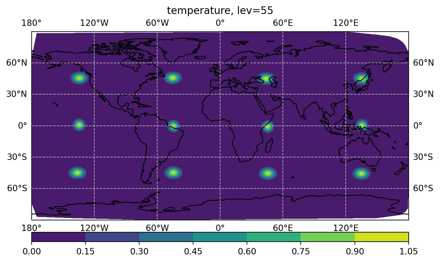
User may play with different localization lengths (e.g., change the horizontal one from 1200km to 2500km) by changing the following YAML keys from bumploc.yaml, then re-submit the PBS job script.

[Note that dirac_nicas.2018-04-15_00.00.00.nc and figure_bumploc.png will be overwritten, so it is a good idea to rename the existing files to compare them to those from a new experiment with modified localization lengths.]

      ...
      io:
	files prefix: bumploc_1200km6km
      ...
      nicas:
        resolution: 8.0
        explicit length-scales: true
        horizontal length-scale:
          - groups: [common]
	    value: 1200.0e3
        vertical length-scale:
          - groups: [common]
	    value: 6.0e3
      ...

Make a plot for Dirac result (with plot_bumploc.py) to see how the localization looks like.

We are now ready to set up and run the first analysis test using 3DEnVar. For this 3DEnVar, we will use a 240 km background forecast and ensemble input at the same resolution.

Let's create a new working directory for this test:

$ cd /glade/derecho/scratch/${USER}/mpas_jedi_tutorial
$ mkdir 3denvar
$ cd 3denvar

Set environment variable for the mpas-bundle directory,

$ export bundle_dir=/glade/derecho/scratch/bjung/mpas_bundle_v4.0.1_public_prebuilt

We can then link the relevant MPAS stream, graph, namelist, and physics files:

$ ln -sf ../MPAS_namelist_stream_physics_files/*BL ./
$ ln -sf ../MPAS_namelist_stream_physics_files/*DATA ./
$ ln -sf ../MPAS_namelist_stream_physics_files/x1.10242.graph.info.part.64 ./
$ ln -sf ../MPAS_namelist_stream_physics_files/namelist.atmosphere_240km ./
$ ln -sf ../MPAS_namelist_stream_physics_files/streams.atmosphere_240km ./
$ ln -sf ../MPAS_namelist_stream_physics_files/stream_list*  ./

Next, we need to link in a few yaml files that define MPAS variables for JEDI:

$ ln -sf ${bundle_dir}/code/mpas-jedi/test/testinput/namelists/geovars.yaml ./
$ ln -sf ${bundle_dir}/code/mpas-jedi/test/testinput/namelists/keptvars.yaml ./
$ ln -sf ${bundle_dir}/code/mpas-jedi/test/testinput/obsop_name_map.yaml ./

Next, we need to link MPAS 2-stream files corresponding to the 240 km mesh. For this experiment we need to link the following files:

$ ln -fs ../MPAS_namelist_stream_physics_files/x1.10242.invariant.nc .
$ ln -fs ../background/2018041418/mpasout.2018-04-15_00.00.00.nc ./templateFields.10242.nc

Next, we should link the background file mpasout.2018-04-15_00.00.00.nc into the working directory and make a copy of the background file as the analysis file to be overwritten.

$ ln -fs ../background/2018041418/mpasout.2018-04-15_00.00.00.nc ./bg.2018-04-15_00.00.00.nc
$ cp ../background/2018041418/mpasout.2018-04-15_00.00.00.nc ./an.2018-04-15_00.00.00.nc

Next, we need to link bump localization files.

$ ln -fs ../localization ./BUMP_files

Next, we need to link observation files into the working directory.

$ ln -fs ../obs_ioda/2018041500/aircraft_obs_2018041500.h5  .
$ ln -fs ../obs_ioda/2018041500/gnssro_obs_2018041500.h5  .
$ ln -fs ../obs_ioda/2018041500/satwind_obs_2018041500.h5  .
$ ln -fs ../obs_ioda/2018041500/sfc_obs_2018041500.h5  .
$ ln -fs ../obs_ioda/2018041500/sondes_obs_2018041500.h5  .

Next, we are ready to link the pre-prepared 3denvar.yaml file for 3DEnVar. 3denvar.yaml contains all of the settings we need for this 3DEnVar update.

$ ln -sf ../MPAS_JEDI_yamls_scripts/3denvar.yaml ./

We are finally ready to link a PBS job script and then submit it. Notice the job script runs the following executable mpasjedi_variational.x, which is used for all of our variational updates.

$ ln -fs ../MPAS_JEDI_yamls_scripts/run_3denvar.csh ./
$ qsub run_3denvar.csh

Once your job is submitted, you can check the status of the job using qstat -u ${USER}. When the job is complete, you can check the log file by using vi mpasjedi_3denvar.log.

Now that the analysis was successful, you may plot the cost function and gradient norm reduction.

$  module load conda
$  conda activate npl
$  cp ${bundle_dir}/code/mpas-jedi/graphics/standalone/plot_cost_grad.py .

Changing 'jedi.log' to 'mpasjedi_3denvar.log' in plot_cost_grad.py, then do

$  python plot_cost_grad.py

You can then view the figure using the following:

$ display costgrad.png

You can also plot the analysis increment (i.e., an.*.nc - bg.*.nc) with the following.

$  cp ../MPAS_JEDI_yamls_scripts/plot_analysis_increment.py ./
$  python plot_analysis_increment.py
$  display figure_increment_uReconstructZonal_10.png

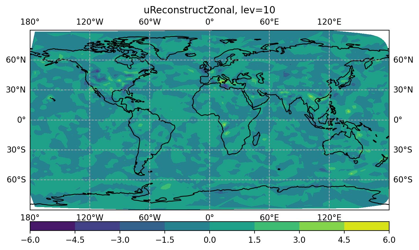
You will also see several so-called DA "feedback" files below:

obsout_da_aircraft.h5
obsout_da_gnssro.h5
obsout_da_satwind.h5
obsout_da_sfc.h5
obsout_da_sondes.h5

You can follow the same procedure as in section 2.4 to plot these 'feedback' files, e.g.,

$ module load conda
$ conda activate npl
$ cp -r ${bundle_dir}/code/mpas-jedi/graphics .
$ cd graphics/standalone
$ python plot_diag.py

This will produce a number of figure files, display one of them

display RMSofOMM_da_aircraft_airTemperature.png

which will look like the figure below

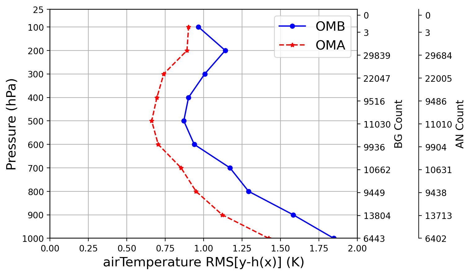
Now we know how to run a 3DEnVar analysis, let's prepare a second test which uses a higher resolution background of 120 km but a coarser ensemble of 240 km.

Let's create a new working directory to run our 120-240km 3DEnVar update:

$ cd /glade/derecho/scratch/${USER}/mpas_jedi_tutorial
$ mkdir 3denvar_120km240km
$ cd 3denvar_120km240km

Set environment variable for the mpas-bundle directory,

$ export bundle_dir=/glade/derecho/scratch/bjung/mpas_bundle_v4.0.1_public_prebuilt

We can then link the relevant MPAS stream, graph, namelist, and physics files. In addition to files for 240km mesh, we also need files for 120 km mesh.

$ ln -sf ../MPAS_namelist_stream_physics_files/*BL ./
$ ln -sf ../MPAS_namelist_stream_physics_files/*DATA ./
$ ln -sf ../MPAS_namelist_stream_physics_files/x1.10242.graph.info.part.64 ./
$ ln -sf ../MPAS_namelist_stream_physics_files/x1.40962.graph.info.part.64 ./
$ ln -sf ../MPAS_namelist_stream_physics_files/namelist.atmosphere_240km ./
$ ln -sf ../MPAS_namelist_stream_physics_files/namelist.atmosphere_120km ./
$ ln -sf ../MPAS_namelist_stream_physics_files/streams.atmosphere_240km ./
$ ln -sf ../MPAS_namelist_stream_physics_files/streams.atmosphere_120km ./
$ ln -sf ../MPAS_namelist_stream_physics_files/stream_list*  ./

Next, we need to link in a few yaml files again that define MPAS variables for JEDI:

$ ln -sf ${bundle_dir}/code/mpas-jedi/test/testinput/namelists/geovars.yaml ./
$ ln -sf ${bundle_dir}/code/mpas-jedi/test/testinput/namelists/keptvars.yaml ./
$ ln -sf ${bundle_dir}/code/mpas-jedi/test/testinput/obsop_name_map.yaml ./

Next, we need to link MPAS 2-stream files corresponding to both 240 km and 120 km MPAS grids. We need both an invariant.nc file and a templateFields.nc file. For this experiment we need to link the following files:

$ ln -fs ../MPAS_namelist_stream_physics_files/x1.10242.invariant.nc .
$ ln -fs ../background/2018041418/mpasout.2018-04-15_00.00.00.nc ./templateFields.10242.nc
$ ln -fs ../MPAS_namelist_stream_physics_files/x1.40962.invariant.nc .
$ ln -fs ../background_120km/2018041418/mpasout.2018-04-15_00.00.00.nc ./templateFields.40962.nc

Next, we should link 120 km background file into the working directory and make a copy of the background file as the analysis file to be overwritten.

$ ln -fs ../background_120km/2018041418/mpasout.2018-04-15_00.00.00.nc ./bg.2018-04-15_00.00.00.nc
$ cp ../background_120km/2018041418/mpasout.2018-04-15_00.00.00.nc ./an.2018-04-15_00.00.00.nc

Next, we need to link our bump localization files.

$ ln -fs ../localization ./BUMP_files

Next, we need to link observation files into the working directory.

$ ln -fs ../obs_ioda/2018041500/aircraft_obs_2018041500.h5  .
$ ln -fs ../obs_ioda/2018041500/gnssro_obs_2018041500.h5  .
$ ln -fs ../obs_ioda/2018041500/satwind_obs_2018041500.h5  .
$ ln -fs ../obs_ioda/2018041500/sfc_obs_2018041500.h5  .
$ ln -fs ../obs_ioda/2018041500/sondes_obs_2018041500.h5  .

Next, we are ready to copy the pre-prepared 3denvar_120km240km.yaml file for this multi-resolution 3DEnVar.

$ ln -sf ../MPAS_JEDI_yamls_scripts/3denvar_120km240km.yaml ./3denvar.yaml

We are finally ready to link a PBS job script and then submit the job.

$ ln -fs ../MPAS_JEDI_yamls_scripts/run_3denvar.csh ./
$ qsub run_3denvar.csh

Again, you can check the status of the job using qstat -u ${USER}. When the job is complete, you can check the log file by using vi mpasjedi_3denvar.log.

Again, you may plot cost function and gradient norm reduction as well as the analysis increment.

You need to change "x1.10242.invariant.nc" to "x1.40962.invariant.nc" within plot_analysis_increment.py in order to plot increment at the 120 km mesh.

Now we know how to run a 3DEnVar analysis, let's try 4DEnVar with 3 subwindows.

Let's create a new working directory to run 240km 4DEnVar:

$ cd /glade/derecho/scratch/${USER}/mpas_jedi_tutorial
$ mkdir 4denvar
$ cd 4denvar

Set environment variable for the mpas-bundle directory,

$ export bundle_dir=/glade/derecho/scratch/bjung/mpas_bundle_v4.0.1_public_prebuilt

We can then link MPAS stream, graph, namelist, and physics files just as we did for 3DEnVar.

$ ln -sf ../MPAS_namelist_stream_physics_files/*BL ./
$ ln -sf ../MPAS_namelist_stream_physics_files/*DATA ./
$ ln -sf ../MPAS_namelist_stream_physics_files/x1.10242.graph.info.part.64 ./
$ ln -sf ../MPAS_namelist_stream_physics_files/namelist.atmosphere_240km ./
$ ln -sf ../MPAS_namelist_stream_physics_files/streams.atmosphere_240km ./
$ ln -sf ../MPAS_namelist_stream_physics_files/stream_list*  ./

Next, we need to link a few yaml files again that define MPAS variables for JEDI:

$ ln -sf ${bundle_dir}/code/mpas-jedi/test/testinput/namelists/geovars.yaml ./
$ ln -sf ${bundle_dir}/code/mpas-jedi/test/testinput/namelists/keptvars.yaml ./
$ ln -sf ${bundle_dir}/code/mpas-jedi/test/testinput/obsop_name_map.yaml ./

Next, we need to link MPAS 2-stream files corresponding to 240km mesh. For this experiment we need to link the following files:

$ ln -fs ../MPAS_namelist_stream_physics_files/x1.10242.invariant.nc .
$ ln -fs ../background/2018041418/mpasout.2018-04-15_00.00.00.nc ./templateFields.10242.nc

Next, we need to link 240km background files for each subwindow into the working directory and make a copy of each background file as the analysis file for each subwindow to be overwritten.

$ ln -fs ../background/2018041418/mpasout.2018-04-14_21.00.00.nc ./bg.2018-04-14_21.00.00.nc
$ cp ../background/2018041418/mpasout.2018-04-14_21.00.00.nc     ./an.2018-04-14_21.00.00.nc
$ ln -fs ../background/2018041418/mpasout.2018-04-15_00.00.00.nc ./bg.2018-04-15_00.00.00.nc
$ cp ../background/2018041418/mpasout.2018-04-15_00.00.00.nc     ./an.2018-04-15_00.00.00.nc
$ ln -fs ../background/2018041418/mpasout.2018-04-15_03.00.00.nc ./bg.2018-04-15_03.00.00.nc
$ cp ../background/2018041418/mpasout.2018-04-15_03.00.00.nc     ./an.2018-04-15_03.00.00.nc

Next, we need to link bump localization files.

$ ln -fs ../localization ./BUMP_files

Next, we need to link observation files.

$ ln -fs ../obs_ioda/2018041500/aircraft_obs_2018041500.h5  .
$ ln -fs ../obs_ioda/2018041500/gnssro_obs_2018041500.h5  .
$ ln -fs ../obs_ioda/2018041500/satwind_obs_2018041500.h5  .
$ ln -fs ../obs_ioda/2018041500/sfc_obs_2018041500.h5  .
$ ln -fs ../obs_ioda/2018041500/sondes_obs_2018041500.h5  .

Next, we are ready to link the pre-prepared 4denvar.yaml file.

$ ln -sf ../MPAS_JEDI_yamls_scripts/4denvar.yaml ./4denvar.yaml

We are finally ready to link a PBS job script and then submit a job. Note that this 4DEnVar job uses 3 nodes with 64 cores per node for 3 subwindows.

$ ln -fs ../MPAS_JEDI_yamls_scripts/run_4denvar.csh ./
$ qsub run_4denvar.csh

Again, you can check the status of the job using qstat -u ${USER}. When the job is complete, you can check the log file by using vi mpasjedi_4denvar.log.

Again, you can plot cost function and gradient norm reduction as well as analysis increments at one of 3 subwindows.

You may modify the an and bg files in plot_analysis_increment.py to see how the increment changes across the subwindows.

In this practice, we will run MPAS-JEDI 3DVar at global 240 km mesh. The overall procedure is similar to the 3D/4DEnVar practice. However, 3DVar uses the static multivariate background error covariance (B), which contains the climatological characteristics. Here, the pre-generated static B will be used. We hope to provide a practice for static B training in future MPAS-JEDI tutorials.

After changing to our /glade/derecho/scratch/${USER}/mpas_jedi_tutorial directory, create the working directory for 3dvar.

$ cd /glade/derecho/scratch/$USER/mpas_jedi_tutorial
$ mkdir 3dvar
$ cd 3dvar

Set environment variable for the mpas-bundle directory,

$ export bundle_dir=/glade/derecho/scratch/bjung/mpas_bundle_v4.0.1_public_prebuilt

Link MPAS physics-related data and tables, MPAS graph, MPAS streams, and MPAS namelist files.

$ ln -fs ../MPAS_namelist_stream_physics_files/*BL ./
$ ln -fs ../MPAS_namelist_stream_physics_files/*DATA ./
$ ln -fs ../MPAS_namelist_stream_physics_files/x1.10242.graph.info.part.64 ./
$ ln -fs ../MPAS_namelist_stream_physics_files/streams.atmosphere_240km ./
$ ln -fs ../MPAS_namelist_stream_physics_files/stream_list.atmosphere.analysis ./
$ ln -fs ../MPAS_namelist_stream_physics_files/stream_list.atmosphere.background ./
$ ln -fs ../MPAS_namelist_stream_physics_files/stream_list.atmosphere.control ./
$ ln -fs ../MPAS_namelist_stream_physics_files/stream_list.atmosphere.ensemble ./
$ ln -fs ../MPAS_namelist_stream_physics_files/namelist.atmosphere_240km ./

Link the background file and copy it as an analysis file.

The file with prefix mpasout contains the variables for "da_state" stream of 2-stream I/O.

And the data assimilation will overwrite several selected analyzed variables (defined in stream_list.atmosphere.analysis) in the analysis file.

$ ln -fs ../background/2018041418/mpasout.2018-04-15_00.00.00.nc ./bg.2018-04-15_00.00.00.nc
$ cp ./bg.2018-04-15_00.00.00.nc ./an.2018-04-15_00.00.00.nc

Link MPAS 2-stream files.

$ ln -fs ../MPAS_namelist_stream_physics_files/x1.10242.invariant.nc .
$ ln -fs ../background/2018041418/mpasout.2018-04-15_00.00.00.nc ./templateFields.10242.nc

Prepare the pre-generated static B files.

$ ln -fs ../B_Matrix ./

Next, link the observation files to be assimilated. Along the conventional observation, here a single AMSU-A radiance observation from NOAA-18 is added.

$ ln -fs ../obs_ioda/2018041500/aircraft_obs_2018041500.h5  .
$ ln -fs ../obs_ioda/2018041500/gnssro_obs_2018041500.h5  .
$ ln -fs ../obs_ioda/2018041500/satwind_obs_2018041500.h5  .
$ ln -fs ../obs_ioda/2018041500/sfc_obs_2018041500.h5  .
$ ln -fs ../obs_ioda/2018041500/sondes_obs_2018041500.h5  .
$ ln -fs ../obs_ioda/2018041500/amsua_n18_obs_2018041500.h5 .

For this 3DVar test, satellite radiance data from NOAA-18's AMSU-A sensor is assimilated, so need coefficient files for CRTM.

$ ln -fs ../crtm_coeffs_v3  ./

Radiance assimilation with VarBC also needs the bias correction files prepared in Section 2.3. Link the coefficients, their error covariance, and the mean temperature lapse rate:

$ ln -fs ../satbias/satbias_amsua_n18.h5      ./
$ ln -fs ../satbias/satbias_cov_amsua_n18.h5  ./
$ ln -fs ../satbias/amsua_n18_tlapmean.txt     ./

VarBC reads these as the a priori coefficients, updates them together with the atmospheric state during the minimization, and writes the updated values to a new file. The relevant keys in 3dvar.yaml are:

    obs bias:
      input file: satbias_amsua_n18.h5
      output file: satbias_amsua_n18_out.h5
      variational bc:
        predictors:
        - name: constant
        - name: lapse_rate
          order: 2
          tlapse: &amsua_n18_tlap amsua_n18_tlapmean.txt
        - name: lapse_rate
          tlapse: *amsua_n18_tlap
        - name: emissivityJacobian
        - name: sensorScanAngle
          order: 4
        - name: sensorScanAngle
          order: 3
        - name: sensorScanAngle
          order: 2
        - name: sensorScanAngle
      covariance:
        minimal required obs number: 20
        variance range: [1.0e-6, 10.0]
        step size: 1.0e-4
        largest analysis variance: 10000.0
        prior:
          input file: satbias_cov_amsua_n18.h5
          inflation:
            ratio: 1.1
            ratio for small dataset: 2.0
        output file: satbias_cov_amsua_n18_out.h5

Link yaml files:

$ ln -fs ${bundle_dir}/code/mpas-jedi/test/testinput/namelists/geovars.yaml  ./
$ ln -fs ${bundle_dir}/code/mpas-jedi/test/testinput/namelists/keptvars.yaml  ./
$ ln -fs ${bundle_dir}/code/mpas-jedi/test/testinput/obsop_name_map.yaml ./
$ ln -sf ../MPAS_JEDI_yamls_scripts/3dvar.yaml ./

Link and submit pbs job script:

$ ln -sf ../MPAS_JEDI_yamls_scripts/run_3dvar.csh ./
$ qsub run_3dvar.csh

User may check the PBS job status by running qstat -u $USER, or monitoring the log file tail -f mpasjedi_3dvar.log .

You may make figures following similar procedures in previous sections.

Once the job finishes, VarBC has written the updated bias coefficients. Compare them against the a priori values from Section 2.3 using the same plotting script:

$ module reset
$ module load conda
$ conda activate npl
$ ln -sf ../MPAS_JEDI_yamls_scripts/plot_satbias.py .
$ python plot_satbias.py satbias_amsua_n18_out.h5
$ display figure_satbias_amsua_n18_out.png

A single 240 km analysis will not move the coefficients very far, but the constant and lapse-rate terms should already show a visible adjustment on the channels with the most observations. The effect of the correction itself is easier to see in observation space: the obsout_da_amsua_n18.h5 feedback file stores both the uncorrected and the bias-corrected departures, so plotting them together shows how much of the mean departure VarBC has removed.

User may want to try additional practice as below.

1. Assimilate additional satellite radiance data.

   To do this, additional obs file (for example, ../obs_ioda/2018041500/amsua_n19_obs_2018041500.h5) should be linked to /glade/derecho/scratch/$USER/mpas_jedi_tutorial/3dvar/, together with the matching satbias files for that sensor, which need to be created following Section 2.3.

   Also, user need to add the corresponding obs space and obs bias yaml keys in 3dvar.yaml.

In this practice, we will run MPAS-JEDI Hybrid-3DEnVar at global 240 km mesh. The hybrid covariance will be made from both static B and ensemble B.

After changing to /glade/derecho/scratch/${USER}/mpas_jedi_tutorial directory, create the working directory for Hybrid-3DEnVar.

$ cd /glade/derecho/scratch/$USER/mpas_jedi_tutorial
$ mkdir hybrid-3denvar
$ cd hybrid-3denvar

Set environment variable for the mpas-bundle directory,

$ export bundle_dir=/glade/derecho/scratch/bjung/mpas_bundle_v4.0.1_public_prebuilt

Link MPAS physics-related data and tables, MPAS graph, MPAS streams, and MPAS namelist files.

$ ln -fs ../MPAS_namelist_stream_physics_files/*BL ./
$ ln -fs ../MPAS_namelist_stream_physics_files/*DATA ./
$ ln -fs ../MPAS_namelist_stream_physics_files/x1.10242.graph.info.part.64 ./
$ ln -fs ../MPAS_namelist_stream_physics_files/streams.atmosphere_240km ./
$ ln -fs ../MPAS_namelist_stream_physics_files/stream_list.atmosphere.analysis ./
$ ln -fs ../MPAS_namelist_stream_physics_files/stream_list.atmosphere.background ./
$ ln -fs ../MPAS_namelist_stream_physics_files/stream_list.atmosphere.control ./
$ ln -fs ../MPAS_namelist_stream_physics_files/stream_list.atmosphere.ensemble ./
$ ln -fs ../MPAS_namelist_stream_physics_files/namelist.atmosphere_240km ./

Link the background file and copy it as an analysis file.

$ ln -fs ../background/2018041418/mpasout.2018-04-15_00.00.00.nc ./bg.2018-04-15_00.00.00.nc
$ cp ./bg.2018-04-15_00.00.00.nc ./an.2018-04-15_00.00.00.nc

Link MPAS 2-stream files.

$ ln -fs ../MPAS_namelist_stream_physics_files/x1.10242.invariant.nc .
$ ln -fs ../background/2018041418/mpasout.2018-04-15_00.00.00.nc ./templateFields.10242.nc

Prepare the pre-generated static B files.

$ ln -fs ../B_Matrix ./

Link the localization files.

$ ln -fs ../localization ./BUMP_files

Link the observation files to be assimilated. Along the conventional observation, here a single AMSU-A radiance observation from NOAA-18 is added.

$ ln -fs ../obs_ioda/2018041500/aircraft_obs_2018041500.h5  .
$ ln -fs ../obs_ioda/2018041500/gnssro_obs_2018041500.h5  .
$ ln -fs ../obs_ioda/2018041500/satwind_obs_2018041500.h5  .
$ ln -fs ../obs_ioda/2018041500/sfc_obs_2018041500.h5  .
$ ln -fs ../obs_ioda/2018041500/sondes_obs_2018041500.h5  .
$ ln -fs ../obs_ioda/2018041500/amsua_n18_obs_2018041500.h5 .

Prepare the coefficient files for CRTM.

$ ln -fs ../crtm_coeffs_v3  ./

Link the bias correction files from Section 2.3, exactly as in Section 5.1.

$ ln -fs ../satbias/satbias_amsua_n18.h5      ./
$ ln -fs ../satbias/satbias_cov_amsua_n18.h5  ./
$ ln -fs ../satbias/amsua_n18_tlapmean.txt     ./

Link yaml files.

$ ln -fs ${bundle_dir}/code/mpas-jedi/test/testinput/namelists/geovars.yaml  ./
$ ln -fs ${bundle_dir}/code/mpas-jedi/test/testinput/namelists/keptvars.yaml  ./
$ ln -fs ${bundle_dir}/code/mpas-jedi/test/testinput/obsop_name_map.yaml ./
$ ln -fs ../MPAS_JEDI_yamls_scripts/3dhyb.yaml ./

Link and submit pbs job script.

$ ln -sf ../MPAS_JEDI_yamls_scripts/run_3dhyb.csh ./
$ qsub run_3dhyb.csh

User may check the PBS job status by running qstat -u $USER, or monitoring the log file tail -f mpasjedi_3dhyb.log .

User may want to try additional practice as below.

1. Change the hybrid weights.

   The default 3dhyb.yaml uses 0.5 and 0.5 weights for static B and ensemble B. User can modify these weights, for example, 0.2/0.8 , 0.8/0.2 , 1.0/0.0 , 0.0/1.0 , or even 2.0/1.5 .

     background error:
       covariance model: hybrid
       components:
       - weight:
       value:  0.5
         covariance:
           covariance model: SABER
           ...
       - weight:
       value:  0.5
         covariance:
           covariance model: ensemble
           ...
   

   You may see some changes in the fit-to-obs statistics, convergence, or analysis increment fields.

2. Compare the VarBC coefficients against those from the 3DVar run in Section 5.1.

   The hybrid background error changes the analysis increment, which in turn changes the departures that VarBC sees. Running plot_satbias.py on both output files shows how much the choice of background error covariance feeds back into the estimated bias.

   $ module reset
   $ module load conda
   $ conda activate npl
   $ ln -sf ../MPAS_JEDI_yamls_scripts/plot_satbias.py .
   $ python plot_satbias.py satbias_amsua_n18_out.h5
   $ display figure_satbias_amsua_n18_out.png
   

The statistics are generated for each cycle and all ObsSpace (e.g., sondes, aircraft, gnssro, etc.) found in the folder containing the data assimilation feedback files (i.e., obsout_da_*.h5). The statistics are binned globally and by latitude bands as specified in config.py. The binned statistics are stored in HDF5 files located in a folder named stats that is created for each cycle. The statistics are generated by the script DiagnoseObsStatistics.py in graphics.

Let's begin by checking the directory called omboma_from2experiments:

$ cd /glade/derecho/scratch/$USER/mpas_jedi_tutorial/omboma_from2experiments

This folder contains sample variational-based DA observation "feedback" files from two experiments Exp1 and Exp2, e.g.,

$ ls Exp1/CyclingDA/*

You will see obsout_da_amsua_n18.h5 and obsout_da_gnssrobndropp1d.h5 under each cycle time during a 2-day period (9 cycles). We can generate the bias, RMSE, and standard deviation statistics of these OMB/OMA files using

$ ln -sf ../MPAS_JEDI_yamls_scripts/generate_stats_omboma.csh .
$ ln -sf ../MPAS_JEDI_yamls_scripts/advanceCYMDH.py .
$ qsub generate_stats_omboma.csh

The job will take ~5 minutes to complete, and you can take a look at the folder of the statistics files:

$ ls Exp1/CyclingDA/*/stats

You will see two files stats_da_amsua_n18.h5 and stats_da_gnssrobndropp1d.h5 in each folder. You may check generate_stats_omboma.csh, in which a line below generated statistical files.

python DiagnoseObsStatistics.py -n ${NUMPROC} -p ${daDiagDir} -o obsout -app variational -nout 1

where

-n: number of tasks/processors for multiprocessing
-p: path to DA feedback files (e.g., Exp1/CyclingDA/2018041500)
-o: prefix for DA feedback files
-app: application (variational or hofx)
-nout: number of outer loops

Also note that advanceCYMDH.py is a python code to help advance the time.

If statistics files were created, we can proceed to make the plots in the next section!

Set environment variable for the mpas-bundle directory,

$ export bundle_dir=/glade/derecho/scratch/bjung/mpas_bundle_v4.0.1_public_prebuilt

Let us make a local copy of the graphics package first:

$ cd /glade/derecho/scratch/$USER/mpas_jedi_tutorial/omboma_from2experiments
$ cp -r ${bundle_dir}/code/mpas-jedi/graphics .
$ cd graphics

Then diff and replace analyze_config.py with a pre-prepared one:

$ diff analyze_config.py ../../MPAS_JEDI_yamls_scripts/analyze_config.py
$ mv analyze_config.py analyze_config.py_default
$ cp ../../MPAS_JEDI_yamls_scripts/analyze_config.py .

You can see the changes made in analyze_config.py by diff. Below provides some explanations about settings in analyze_config.py.

• Set the first and last cycle date time:

  dbConf['firstCycleDTime'] = dt.datetime(2018,4,15,0,0,0)
  dbConf['lastCycleDTime'] = dt.datetime(2018,4,17,0,0,0)

• Set the time increment between valid date times to 6 hours:

  dbConf['cyTimeInc'] = dt.timedelta(hours=6)

• Set the verification type to omb/oma:

  VerificationType = 'omb/oma'

• Set the verification space to obs:

  VerificationSpace = 'obs'

• Set the workflow type to MPAS-JEDI_tutorial:

  workflowType = 'MPAS-JEDI_tutorial'
  

• Set the path to the experiment's folder:

  dbConf['expDirectory'] = os.getenv('EXP_DIR','/glade/derecho/scratch/'+user+'/mpas_jedi_tutorial/omboma_from2experiments')

• Set the the name of the experiment that will be used as reference or control:

  dbConf['cntrlExpName'] = 'exp1'

• Specify the experiments to be analyzed. Make sure that the value given to cntrlExpName is one of the keys in the dictionary experiments:

  experiments['exp1'] = 'Exp1' + deterministicVerifyDir
  experiments['exp2'] = 'Exp2' + deterministicVerifyDir

Last, setting python environment and do

$ module reset
$ module load conda
$ conda activate npl

$ ./SpawnAnalyzeStats.py -a UMMM0016 -app variational -nout 1 -d gnssrobndropp1d
$ ./SpawnAnalyzeStats.py -a UMMM0016 -app variational -nout 1 -d amsua_n18

Each SpawnAnalyzeStats.py command triggers two PBS jobs for making two types of figures under gnssrobndropp1d_analyses and amsua_n18_analyses directories.

• BinValAxisProfileDiffCI: vertical profiles of RMS relative differences from the RMS of OmB of Exp1 with confidence intervals (95%), as a function of the impact height for different latitude bands and binned by latitude at 10km
  CYAxisExpLines: time series of the bias, count, RMS, and STD averaged globally and by latitude bands
  

SpawnAnalyzeStats.py can take some arguments (similar as in previous section), such as:

-a: account
-app: application (e.g., variational, hofx)
-nout: number of outer loops in the variational method
-d: diagSpaces (e.g., amsua_,sonde,airc,sfc,gnssrobndropp1d,satwind)

After jobs complete, you may check gnssrobndropp1d_analyses/CYAxisExpLines/omm, for example,

$ cd gnssrobndropp1d_analyses/CYAxisExpLines/omm
$ display QCflag_good_TSeries_0min_gnssrobndropp1d_omm_RMS.pdf

which will look like the figure below

To view more figures, it is more convenient to transfer them to your local computer via:

$ scp -r $USER@data-access.ucar.edu:/glade/derecho/scratch/$USER/mpas_jedi_tutorial/omboma_from2experiments/graphics/gnssrobndropp1d_analyses .
$ scp -r $USER@data-access.ucar.edu:/glade/derecho/scratch/$USER/mpas_jedi_tutorial/omboma_from2experiments/graphics/amsua_n18_analyses .

In this practice, we will run MPAS-JEDI 3DEnVar at a regional 15 km mesh.

The regional MPAS-JEDI test is under conus15km, where all necessary input files are already prepared. You can simply submit a job script with:

$ cd /glade/derecho/scratch/$USER/mpas_jedi_tutorial/conus15km
$ qsub run_conus15km.csh

Before running the job script, let's take a closer look at namelist.atmosphere, streams.atmosphere, and 3denvar.yaml under conus15km. There are a large number of settings in these files, but only a few sections need your attention to go from a global to a regional configuration.

In namelist.atmosphere, the &limited_area block must apply the lateral boundary conditions:

&limited_area
    config_apply_lbcs = true
/

In streams.atmosphere, an lbc_in immutable stream must be declared:

<immutable_stream name="lbc_in"
                  type="input"
                  io_type="pnetcdf,cdf5"
                  filename_template="lbc.$Y-$M-$D_$h.$m.$s.nc"
                  filename_interval="input_interval"
                  packages="limited_area"
                  input_interval="3:00:00" />

Finally, in 3denvar.yaml, under the obs filters: section, we use a Bounds Check filter to reject observations that fall outside the regional domain. Here we use the ObsFunction/LAMDomainCheck, which defines a circular domain via a central latitude/longitude and a radius:

- filter: Bounds Check
  filter variables:
  - name: airTemperature
  - name: windEastward
  - name: windNorthward
  - name: specificHumidity
  test variables:
  - name: ObsFunction/LAMDomainCheck
    options:
      map_projection: circle    # an option currently supported
      save: true                # will save the DerivedValue to IODA output file
      cenlat: 45.0              # central lat
      cenlon: 278.0             # central lon
      radius: 1820.0            # km
  minvalue: 1.0   # will filter all obs outside of the specified limited area domain

This filter rejects any observation reported outside of the specified circular domain (centered at 45°N, 278°E with a 1820 km radius, in this test case).

After checking the files namelist.atmosphere, streams.atmosphere, and 3denvar.yaml, we can submit the job script with:

$ qsub run_conus15km.csh

The LAMDomainCheck filter above only supports a circular domain. There is another, more generic way to do regional obs filtering that works for any domain shape. You can try replacing the Bounds Check filter in 3denvar.yaml with the following:

- filter: Bounds Check
  filter variables:
  - name: airTemperature
  - name: windEastward
  - name: windNorthward
  - name: specificHumidity
  test variables:
  - name: GeoVaLs/observable_domain_mask
  flag all filter variables if any test variable is out of bounds: true
  minvalue: 0.0
  maxvalue: 0.1

After editing 3denvar.yaml, resubmit the job script to rerun the analysis with this alternative filter:

$ qsub run_conus15km.csh

Once the job completes, we can check the observation-space diagnostics by copying plot_diag_regional_tut.py to your working directory and running it:

$ module load conda
$ conda activate npl
$ cp ../MPAS_JEDI_yamls_scripts/plot_diag_regional_tut.py .
$ python plot_diag_regional_tut.py

For each assimilated radiosonde variable (airTemperature, windEastward, windNorthward, specificHumidity), the script reads the ombg (observation-minus-background) and oman (observation-minus-analysis) departures from obsout_da_sondes.h5.

This produces one figure per variable:

omb_oma_regional_airTemperature.png
omb_oma_regional_windEastward.png
omb_oma_regional_windNorthward.png
omb_oma_regional_specificHumidity.png

Display one of them, for example:

$ display omb_oma_regional_windEastward.png

Let’s begin by setting up the folder structure needed for the cycling experiment. Within the mpas_jedi_tutorial directory, create a new directory named 3dvarCyclingDA to set up the data assimilation (DA) experiment for 0000 UTC on 15 April 2018 and run a forecast from the generated analysis. This experiment will use MPAS-JEDI with the 3DVar configuration on a global 240 km mesh. Additionally, create subdirectories for the DA and executing the 6-hour MPAS-A forecasts during each cycle.

$ export mpasjedi_tutorial=/glade/derecho/scratch/${USER}/mpas_jedi_tutorial
$ cd ${mpasjedi_tutorial}
$ mkdir 3dvarCyclingDA
$ cd 3dvarCyclingDA
$ mkdir CyclingFC
$ mkdir CyclingDA

For the analysis at 0000 UTC 15 April 2018, we need a 6-hour MPAS-A forecast initialized at 1800 UTC on 14 April 2018 to serve as the background. To generate this forecast, we'll apply the methods learned in the MPAS-A tutorial—using GFS initial conditions along with a pre-generated invariant file that contains all time-invariant fields.

Navigate to the CyclingFC directory and create a folder named 2018041418 for the first cycle date:

$ cd CyclingFC
$ mkdir 2018041418
$ cd 2018041418

For later substitutions in the configuration YAML file, we construct the corresponding date and time strings in the required formats.

$ export thisValidDate=2018041418
$ export thisMPASFileDate=2018-04-14_18.00.00
$ export thisMPASNamelistDate=2018-04-14_18:00:00
$ export nextMPASFileDate=2018-04-15_00.00.00

Link the invariant file and the GFS initial conditions on the MPAS-A mesh into the cycle directory and create a symbolic link to the appropriate init file that will be used to update sea surface temperature (SST) and sea-ice fractional area coverage (XICE). These init files, used for surface updates, have been pre-generated using methods covered in the MPAS-A tutorial. Specifically, the invariant file was placed in the "input" stream, and the "filename_template" for the "output" stream was set to produce the init files (details not covered here).

$ ln -sf ${mpasjedi_tutorial}/MPAS_namelist_stream_physics_files/x1.10242.invariant.nc .
$ ln -sf ${mpasjedi_tutorial}/cyclingDA/init/${thisValidDate}/x1.10242.init.${thisMPASFileDate}.nc ./mpasin.${thisMPASFileDate}.nc
$ ln -sf ${mpasjedi_tutorial}/cyclingDA/init/${thisValidDate}/x1.10242.init.${thisMPASFileDate}.nc ./x1.10242.sfc_update.nc

Link MPAS physics-related data and tables, MPAS-A graph, MPAS-A streams, and MPAS-A namelist files:

$ ln -sf ${mpasjedi_tutorial}/MPAS_namelist_stream_physics_files/*BL ./
$ ln -sf ${mpasjedi_tutorial}/MPAS_namelist_stream_physics_files/*DATA ./
$ ln -sf ${mpasjedi_tutorial}/MPAS_namelist_stream_physics_files/x1.10242.graph.info.part.64 ./
$ cp -v ${mpasjedi_tutorial}/cyclingDA/namelist.atmosphere_240km ./namelist.atmosphere
$ ln -sf ${mpasjedi_tutorial}/cyclingDA/streams.atmosphere_240km ./streams.atmosphere
$ ln -sf ${mpasjedi_tutorial}/cyclingDA/stream_list*  ./

Note that we use the "invariant" and "da_state" streams in streams.atmosphere.

immutable_stream name="invariant"
                  type="input"
                  precision="single"
                  filename_template="x1.10242.invariant.nc"
                  io_type="pnetcdf,cdf5"
                  input_interval="initial_only"

immutable_stream name="da_state"
                  type="output"
                  precision="single"
                  clobber_mode="truncate"
                  filename_template="mpasout.$Y-$M-$D_$h.$m.$s.nc"
                  packages="jedi_da"
                  io_type="pnetcdf,cdf5"
                  output_interval="06:00:00"

Also, note that config_jedi_da is set to True in namelist.atmosphere. For cold-start model runs config_do_DAcycling needs to be set to False, set configDODACycling to False and make the variable substitution in the namelist. Also, substitute the start time in the namelist.

$ export configDODACycling=false
$ sed -i 's@{{configDODACycling}}@'${configDODACycling}'@g' namelist.atmosphere
$ sed -i 's@{{startTime}}@'${thisMPASNamelistDate}'@g' namelist.atmosphere

Now, run the model submitting a job with qsub, but first copy the prepared job script to the working directory.

$ ln -sf ${mpasjedi_tutorial}/cyclingDA/run_model.pbs .
$ qsub run_model.pbs

You can monitor the status of the job using qstat -u ${USER}, and follow the model's progress in real time with tail -f log.atmosphere.0000.out. At this resolution, the model runs quite fast, so you should see it complete shortly. Once finished, the output directory will contain the expected mpasout files for the 0- and 6-hour forecasts:

$ ls -l mpasout.*

With the 6-hour background already generated, we're now ready to begin the DA cycle. Navigate to the CyclingDA directory and create a folder for the current cycle.

$ cd ${mpasjedi_tutorial}/3dvarCyclingDA/CyclingDA
$ mkdir 2018041500
$ cd 2018041500

For later substitutions in the configuration YAML file, we define several date related variables, including the current valid time, the previous valid time, and the initial time of the DA time window. We then construct the corresponding date and time strings in the required formats.

$ export prevValidDate=2018041418
$ export thisValidDate=2018041500
$ export thisFileDate=2018-04-15T00:00:00
$ export thisMPASFileDate=2018-04-15_00.00.00
$ export thisMPASNamelistDate=2018-04-15_00:00:00
$ export halfprevDate=2018-04-14T21:00:00
$ export nextMPASFileDate=2018-04-15_06.00.00

Now, follow similar steps as outlined in Section 5.1, but this time for the 3DVar configuration. Link the required files, including MPAS-A physics data and tables, the MPAS-A graph file, streams configuration, and namelist files.

$ ln -sf ${mpasjedi_tutorial}/MPAS_namelist_stream_physics_files/*BL ./
$ ln -sf ${mpasjedi_tutorial}/MPAS_namelist_stream_physics_files/*DATA ./
$ ln -sf ${mpasjedi_tutorial}/MPAS_namelist_stream_physics_files/x1.10242.graph.info.part.64 ./
$ cp -v ${mpasjedi_tutorial}/cyclingDA/namelist.atmosphere_240km ./
$ ln -sf ${mpasjedi_tutorial}/MPAS_namelist_stream_physics_files/streams.atmosphere_240km ./
$ ln -sf ${mpasjedi_tutorial}/MPAS_namelist_stream_physics_files/stream_list*  ./

For cycling DA runs config_do_DAcycling needs to be set to true, thus, set the variable configDODACycling to True and make the variable substitution in the namelist. In addition, substitute the start date entry in the namelist file to match the current cycle.

$ export configDODACycling=true
$ sed -i 's@{{configDODACycling}}@'${configDODACycling}'@g' namelist.atmosphere_240km
$ sed -i 's@{{startTime}}@'${thisMPASNamelistDate}'@g' namelist.atmosphere_240km

Link the background file mpasout.${thisMPASFileDate}.nc into the working directory, and make a copy of it to serve as the analysis file, which will be overwritten during the DA step.

$ ln -fs ../../CyclingFC/${prevValidDate}/mpasout.${thisMPASFileDate}.nc ./bg.${thisMPASFileDate}.nc
$ cp -v ../../CyclingFC/${prevValidDate}/mpasout.${thisMPASFileDate}.nc ./an.${thisMPASFileDate}.nc

Link MPAS-A 2-stream I/O files corresponding to the 240 km mesh.

$ ln -fs ${mpasjedi_tutorial}/MPAS_namelist_stream_physics_files/x1.10242.invariant.nc .
$ ln -fs ../../CyclingFC/${prevValidDate}/mpasout.${thisMPASFileDate}.nc ./templateFields.10242.nc

Note that the templateFields file is used as the "input" stream in streams.atmosphere.

immutable_stream name="input"
                  type="input"
                  precision="single"
                  filename_template="templateFields.10242.nc"
                  io_type="pnetcdf,cdf5"
                  input_interval="initial_only"

Link the pre-generated static B files.

$ ln -fs ${mpasjedi_tutorial}/B_Matrix ./

Link the observation files to be assimilated.

$ ln -fs ${mpasjedi_tutorial}/obs_ioda/${thisValidDate}/aircraft_obs_${thisValidDate}.h5  .
$ ln -fs ${mpasjedi_tutorial}/obs_ioda/${thisValidDate}/gnssro_obs_${thisValidDate}.h5  .
$ ln -fs ${mpasjedi_tutorial}/obs_ioda/${thisValidDate}/satwind_obs_${thisValidDate}.h5  .
$ ln -fs ${mpasjedi_tutorial}/obs_ioda/${thisValidDate}/sfc_obs_${thisValidDate}.h5  .
$ ln -fs ${mpasjedi_tutorial}/obs_ioda/${thisValidDate}/sondes_obs_${thisValidDate}.h5  .
$ ln -fs ${mpasjedi_tutorial}/obs_ioda/${thisValidDate}/amsua_n18_obs_${thisValidDate}.h5 .

Link the coefficient files for CRTM.

$ ln -fs ${mpasjedi_tutorial}/crtm_coeffs_v3  ./

Link the bias correction files. In a cycling experiment the bias coefficients are part of the cycled state: each analysis reads the coefficients written by the previous cycle. For this first cycle there is no previous analysis, so we start from the files prepared in Section 2.3.

$ ln -fs ${mpasjedi_tutorial}/satbias/satbias_amsua_n18.h5      ./
$ ln -fs ${mpasjedi_tutorial}/satbias/satbias_cov_amsua_n18.h5  ./
$ ln -fs ${mpasjedi_tutorial}/satbias/amsua_n18_tlapmean.txt     ./

For the second and later cycles, replace the first two links with the output files from the previous cycle, i.e. ../${prevValidDate}/satbias_amsua_n18_out.h5 (linked as satbias_amsua_n18_out.h5). This is what {{prevDate}} is substituted for in 3dvar_cyclingDA.yaml below.

Link YAML files that define MPAS-A variables for JEDI.

$ export bundle_dir=/glade/derecho/scratch/bjung/mpas_bundle_v4.0.1_public_prebuilt
$ ln -fs ${bundle_dir}/code/mpas-jedi/test/testinput/namelists/geovars.yaml  ./
$ ln -fs ${bundle_dir}/code/mpas-jedi/test/testinput/namelists/keptvars.yaml  ./
$ ln -fs ${bundle_dir}/code/mpas-jedi/test/testinput/obsop_name_map.yaml ./

Next, we are ready to copy the template 3dvar_cyclingDA.yaml file for 3DVar and make the following substitutions:

$ cp -v ${mpasjedi_tutorial}/cyclingDA/3dvar_cyclingDA.yaml ./
$ sed -i 's@{{prevDate}}@'${prevValidDate}'@g' 3dvar_cyclingDA.yaml
$ sed -i 's@{{thisValidDate}}@'${thisValidDate}'@g' 3dvar_cyclingDA.yaml
$ sed -i 's@{{thisFileDate}}@'${thisFileDate}'@g' 3dvar_cyclingDA.yaml
$ sed -i 's@{{thisMPASFileDate}}@'${thisMPASFileDate}'@g' 3dvar_cyclingDA.yaml
$ sed -i 's@{{begin}}@'${halfprevDate}'@g' 3dvar_cyclingDA.yaml

Link and submit pbs job script.

$ ln -sf ${mpasjedi_tutorial}/cyclingDA/run_3dvar.csh ./
$ qsub run_3dvar.csh

You can check the PBS job status using qstat -u $USER, or monitor its progress in real time by running tail -f mpasjedi_3dvar.log.

Once the job finishes, you may want to check the changes in the fit-to-obs statistics, convergence, or analysis increment fields, following similar procedures as in previous sections. VarBC will have written the updated bias coefficients. You can compare them against the a priori values from Section 5.1 and 5.2 using the same plotting script:

$ module reset
$ module load conda
$ conda activate npl
$ ln -sf ../../../MPAS_JEDI_yamls_scripts/plot_satbias.py .
$ python plot_satbias.py satbias_amsua_n18_out.h5
$ display figure_satbias_amsua_n18_out.png

After the analysis step completes successfully, the updated analysis file is used as the initial condition to run MPAS-A and generate the next 6-hour forecast. To proceed, navigate to the CyclingFC directory and create a subdirectory for the current cycle, named 2018041500.

$ cd ${mpasjedi_tutorial}/3dvarCyclingDA/CyclingFC
$ mkdir ${thisValidDate}
$ cd ${thisValidDate}

Link the analysis file and rename it to mpasin.

$ ln -sf ../../CyclingDA/${thisValidDate}/an.${thisMPASFileDate}.nc mpasin.${thisMPASFileDate}.nc

Link MPAS-A physics-related data and tables, MPAS-A graph, MPAS-A streams, and MPAS-A namelist files.

$ ln -sf ${mpasjedi_tutorial}/MPAS_namelist_stream_physics_files/*BL ./
$ ln -sf ${mpasjedi_tutorial}/MPAS_namelist_stream_physics_files/*DATA ./
$ ln -sf ${mpasjedi_tutorial}/MPAS_namelist_stream_physics_files/x1.10242.graph.info.part.64 ./
$ cp -v ${mpasjedi_tutorial}/cyclingDA/namelist.atmosphere_240km ./namelist.atmosphere
$ ln -sf ${mpasjedi_tutorial}/cyclingDA/streams.atmosphere_240km ./streams.atmosphere
$ ln -sf ${mpasjedi_tutorial}/cyclingDA/stream_list*  ./

For warm-start model runs set the variable configDODACycling to True and make the variable substitution in the namelist. Also, substitute the start time in the namelist.

$ export configDODACycling=true
$ sed -i 's@{{configDODACycling}}@'${configDODACycling}'@g' namelist.atmosphere
$ sed -i 's@{{startTime}}@'${thisMPASNamelistDate}'@g' namelist.atmosphere

Link the invariant file and GFS initial conditions on the MPAS-A mesh for this current cycle and create a link of the init file to be used for sea-surface temperature and fractional area coverage of sea-ice update:

$ ln -sf ${mpasjedi_tutorial}/MPAS_namelist_stream_physics_files/x1.10242.invariant.nc .
$ ln -sf ${mpasjedi_tutorial}/cyclingDA/init/${thisValidDate}/x1.10242.init.${thisMPASFileDate}.nc ./
$ ln -sf ${mpasjedi_tutorial}/cyclingDA/init/${thisValidDate}/x1.10242.init.${thisMPASFileDate}.nc ./x1.10242.sfc_update.nc

Run the model submitting a job with qsub, but first copy the prepared job script to the working directory.

$ ln -sf ${mpasjedi_tutorial}/cyclingDA/run_model.pbs .
$ qsub run_model.pbs

Again, monitor the status of the job by issuing qstat -u ${USER} and follow the progress of the model run with tail -f log.atmosphere.0000.out. Once the model has finished successfully, we should see the following mpasout files in the directory for the 0- and 6-h forecast:

$ ls -l mpasout.*

Once the 6-hour forecast is generated, subsequent cycles are similar to the first one. And with that, we have completed a one-cycle data assimilation experiment!!!

Let's reset some module environment and move to the working directory.

$ module reset
$ module load conda
$ conda activate npl
$ module load ncl

$ cd /glade/derecho/scratch/$USER/mpas_jedi_tutorial/Bflow_preprocessing

Users will see the five shell scripts, which do smaller steps. The major step will be 3_convert_uv_to_psichi.bash, but other steps are also included here to simplify the following subsection.

$ bash 1_generate_ESMF_weights.bash

This script will generate the NetCDF files of ESMF interpolation weights between MPAS mesh (global quasi uniform 120 km in this hands-on) and regular latitude-longitude grids (1 degree in this hands-on) via NCL. Two interpolation weight files will be generated ( both directions; from MPAS to lat/lon; from lat/lon to MPAS) as follow:

ESMF_weights/latlon_1p0_to_MPAS_x1.10242_bilinear.nc
ESMF_weights/MPAS_x1.10242_to_latlon_1p0_bilinear.nc

$ bash 2_generate_template_PTB.bash

This script will generate a template file only including “stream_function” and “velocity_potential” via NCO commands. This is especially convenient when we work with a large size of file.

template_PTB.nc

$ bash 3_convert_uv_to_psichi.bash 24
$ bash 3_convert_uv_to_psichi.bash 48

This script will convert the zonal and meridional winds at MPAS cell center into stream function and velocity_potential via NCL. The zonal and meridional winds on the MPAS mesh will be interpolated to lat/lon grid, then converted as “stream_function” and velocity potential with “uv2sfvpf“ function. Then, the stream_function and velocity_potential on the 1 degree lat/lon grid will be interpolated back to MPAS mesh.

This will be performed across range of model initialization time (from 2018040100 to 2018043000 with 12 hour interval in this hands-on example) for two different forecast lead times (24 hr and 48 hr). To use the computing resource more efficiently, multiple NCL executions are performed with a PBS job script. Users can find the outputs as follow:

output/YYYYMMDDHH/FULL_f24.nc   # 24 hour forecast lead time
output/YYYYMMDDHH/FULL_f48.nc   # 48 hour forecast lead time

Here, YYYYMMDDHH represents the model valid time. At this point, FULL_fHH.nc files only contain two full field variables, which are “steram_function” and “velocity_potential".

$ bash 4_add_variables.bash 24
$ bash 4_add_variables.bash 48

This step adds additional variables to FULL_fXX.nc files with NCO commands.

“Temperature” and “spechum" are converted from other variables that are available from MPAS initial files, while “surface_pressure” is directly added. “uReconstructZonal,uReconstructMeridional” are added in case user may want generate the univariate B statistics. Users may also add the cloud hydrometeor variables if they are available.

This will be performed across range of model initialization time (from 2018040100 to 2018043000 with 12 hour interval in this hands-on example) for two different forecast lead times (24 hr and 48 hr). To use the computing resource more efficiently, multiple bash shell scripts are executed with a PBS job script. Users can find the outputs as follow:

output/YYYYMMDDHH/FULL_f24.nc   # 24 hour forecast lead time
output/YYYYMMDDHH/FULL_f48.nc   # 48 hour forecast lead time

Here, YYYYMMDDHH represents the model valid time. At this point, FULL_fHH.nc files contain the following full field variables: “steram_function”, “velocity_potential”, “temperature”, “spechum”, “surface_pressure”, and (optionally) uReconstructZonal,uReconstructMeridional, relhum, qc, qi, qr, qs, qg.

$ bash 5_ncdiff.bash

In this step, the purturbation files are generated by subtracting the full fields of 24 hour forecast lead time from the full fields of 48 hour forecast lead time with NCO commands. These perturbation files will be used in the next section for further B training.

This will be performed across range of model **valid** times (from 2018040300 to 2018050100 with 12 hour interval in this hands-on example). To use the computing resource more efficiently, multiple bash shell scripts are executed with a PBS job script. Users can find the outputs as follow:

output/YYYYMMDDHH/PTB_f48mf24.nc

Here, YYYYMMDDHH represents the model valid time.

$ cd /glade/derecho/scratch/$USER/mpas_jedi_tutorial/Bflow_global240km

Users can find several shell scripts, which do smaller steps, and plot_diagnostics directory, which includes several diagnostic scripts.

$ bash 0_link_samples.bash

While the B training yaml files can handle the list of training sample files (this can be several hundreds of lines), it is convenient to link the training samples, generated from previous section, as an ordered file name as follows

samples/PTB_f48mf24_###.nc   #where ### represent the given index, sequentially from 001 to total number of samples.

$ bash 1_run_vbal.bash

This step reads the training samples (under samples directory), calculates the vertical regression coefficients between the desirable variables. It uses the MPAS-JEDI executable, mpasjedi_error_covariance_toolbox.x. Users will see the following major output files.

VBAL/mpas_vbal_local_000064-0000##.nc      : local regression coefficient files for each processor
VBAL/mpas_sampling_local_000064-0000##.nc  : local sampling files for each processor
VBAL/mpas_vbal.nc                          : global regression coefficient file
VBAL/mpas_sampling.nc                      : global sampling file

Users can make a plot for diagnosed vertical regression coefficients.

$ cd /glade/derecho/scratch/$USER/mpas_jedi_tutorial/Bflow_global240km/plot_diagnostics
$ ncl plot_vbal_regcoef.ncl
$ display -rotate 270 plot_vbal_regcoef_150.pdf

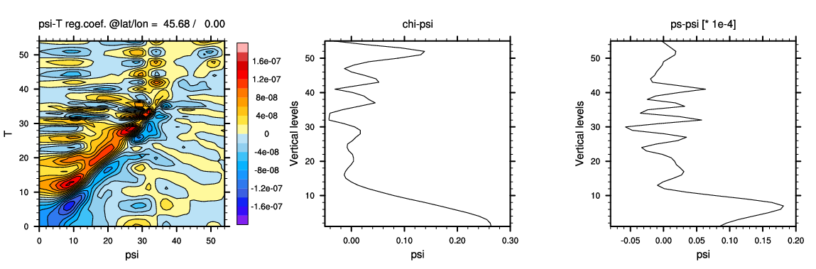
$ ncl plot_vbal_explained_variance.ncl
$ display -rotate 270 plot_vbal_explained_variance.pdf

$ cd /glade/derecho/scratch/$USER/mpas_jedi_tutorial/Bflow_global240km
$ bash 2a_run_hdiag_var.bash

This step reads the training samples (under samples directory) of {stream_function, velocity_potential, temperature, specific humidity, surface_pressure}, applies the inverse operator of BUMP Vertical Balance (which gives the unbalanced samples of {stream_function, unbalanced velocity_potential, unbalanced temperature, specific humidity, unbalanced surface_pressure}), calculates and writes out three B parameters, which are the error standard deviation, horizontal and vertical correlation lengths. It uses the MPAS-JEDI executable, mpasjedi_error_covariance_toolbox.x. Users will see the following major output files.

HDIAG_VAR/vargroup1/mpas.cor_rh.nc
HDIAG_VAR/vargroup1/mpas.cor_rv.nc
HDIAG_VAR/vargroup1/mpas.stddev.nc

Users will find the similar script, 2b_run_hdiag_var.bash, for cloud hydrometeor variables.

$ bash 2c_modify_diagnostics.bash

This step performs several manipulations to the diagnosed B parameter files.

• If there exist separate diagnostic files, it is convenient to merge those into a single file.
• If the diagnostics for cloud hydrometer variables contains missing values, it is replaced by “0.0” values for further processing (see etc_modify_missing.bash).
• If needed, the diagnosed B parameters are modified. In this hands-on, the horizontal correlation lengths for stream function and unbalanced velocity_potential is reduced by a factor of 2 (see etc_modify_cor.bash). Also, the standard deviations for all variables are reduced by a factor of 3 (see etc_modify_var.bash).

Users will find the results as follow:

HDIAG_VAR/merge/mpas.cor_rh.nc
HDIAG_VAR/merge/mpas.cor_rv.nc
HDIAG_VAR/merge/mpas.stddev.nc

Users can make a plot for diagnosed (and modified) B parameters.

$ cd /glade/derecho/scratch/$USER/mpas_jedi_tutorial/Bflow_global240km/plot_diagnostics
$ python plot_B_param_cor_rh.py
$ display plot_B_param_cor_rh.png

$ python plot_B_param_cor_rv.py
$ display plot_B_param_cor_rv.png

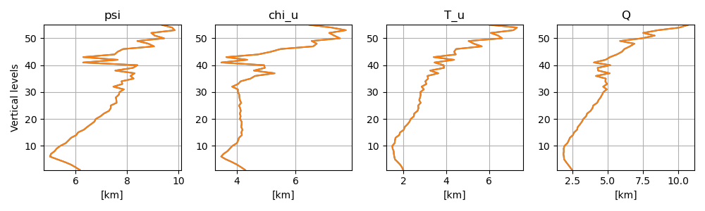
$ python plot_B_param_stddev.py
$ display plot_B_param_stddev.png

$ cd /glade/derecho/scratch/$USER/mpas_jedi_tutorial/Bflow_global240km
$ bash 3_run_nicas_split.bash

This step calculates the spatial correlation by reading the diagnosed horizontal and vertical correlation length files (i.e., mpas.cor_rh.nc and mpas.cor_rv.nc). Because the executaion can take significantly long time in some cases, this step is separately done for each variable. It uses the MPAS-JEDI executable, mpasjedi_error_covariance_toolbox.x. Users will see the following major output files.

NICAS.split/{varname}/mpas_nicas_local_000064-0000##.nc  : local NICAS files for each processor
NICAS.split/{varname}/mpas_nicas.nc                      : global NICAS files
NICAS.split/{varname}/mpas.dirac_nicas.nc                : fields of BUMP-Dirac test

$ bash 4_merge_nicas.bash

This step merged the NICAS files generated in the previous section (for individual variable) into a single file with NCO commands. Users can find the merged files as follow:

NICAS.split/merge/mpas_nicas_local_000064-0000##.nc  : local NICAS files for each processor
NICAS.split/merge/mpas_nicas.nc                      : global NICAS files
NICAS.split/merge/mpas.dirac_nicas.nc                : fields of BUMP-Dirac test

Users can make a plot for the fields of Dirac test. Note that these Dirac test shows the univariate structure for each individual variable.

$ cd /glade/derecho/scratch/$USER/mpas_jedi_tutorial/Bflow_global240km/plot_diagnostics
$ ncl plot_dirac_nicas_group1.ncl
$ display -rotate 270 plot_dirac_nicas_group1.pdf

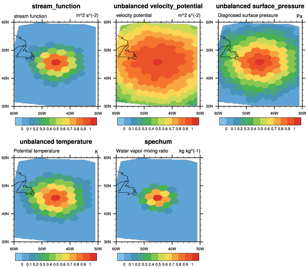
Now users have generated all necessary files for multivariate static background error covariance. The essential files for actual 3DVar or Hybrid-3DEnVar are as follows.

VBAL/mpas_vbal_local_000064-0000##.nc      : local regression coefficient files for each processor
VBAL/mpas_sampling_local_000064-0000##.nc  : local sampling files for each processor
HDIAG_VAR/merge/mpas.stddev.nc
NICAS.split/merge/mpas_nicas_local_000064-0000##.nc  : local NICAS files for each processor

Users can explore the effect of multivariate B with a single observation test. Here, only two observations, one for temperature and the other for zonal wind, are assimilated with the executable mpasjedi_variational.x.

$ cd /glade/derecho/scratch/$USER/mpas_jedi_tutorial/Bflow_global240km
$ bash 5_SO.bash

Like the previous variational practices, users can find the output (i.e., analysis file) from SO/an.2018-04-15_00.00.00.nc. Users can make a plot for the analysis increment fields, focused on the two observation locations.

$ cd /glade/derecho/scratch/$USER/mpas_jedi_tutorial/Bflow_global240km/plot_diagnostics
$ ncl plot_SO_T.ncl
$ display plot_SO_T.pdf

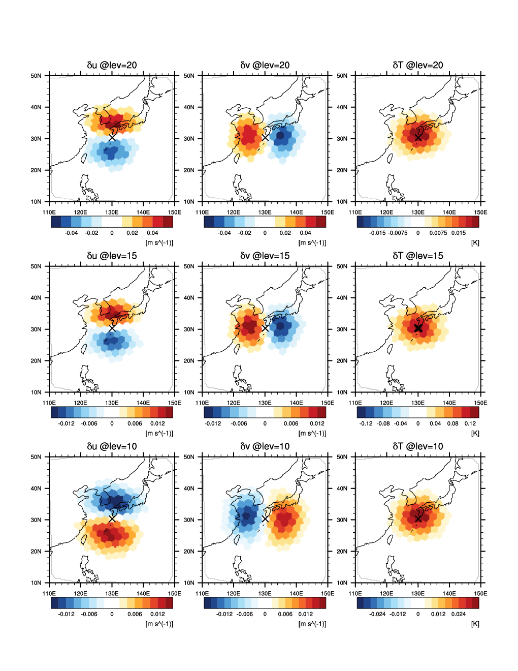
$ ncl plot_SO_U.ncl
$ display plot_SO_U.pdf

The observation can be configured directly from the yaml. For example, users may test different locations ("lats", "lons", "vert coords") or different "obs values" and "obs errors".

  observations:
    observers:
    - obs space:
        name: SO_T
        simulated variables: [airTemperature]
        obsdatain:
          engine:
            type: GenList
            lats: [30.3061]
            lons: [130.085]
            vert coord type: pressure
            vert coords: [78775.95]
            dateTimes: [0]
            epoch: "seconds since 2018-04-15T00:00:00Z"
            obs errors: [0.8]
            obs values: [284.5912]
        obsdataout:
          engine:
            type: H5File
            obsfile: ./obsout_SO_T.h5
      obs operator:
        name: VertInterp
      #obs filters:
      #- filter: GOMsaver
      #  filename: ./geoval_SO_T.nc4
    - obs space:
        name: SO_U
        simulated variables: [windEastward]
        obsdatain:
          engine:
            type: GenList
            lats: [57.7699]
            lons: [357.713]
            vert coord type: pressure
            vert coords: [77693.09]
            dateTimes: [0]
            epoch: "seconds since 2018-04-15T00:00:00Z"
            obs errors: [1.0]
	    obs values: [0.7250047]
        obsdataout:
          engine:
            type: H5File
            obsfile: ./obsout_SO_U.h5
      obs operator:
        name: VertInterp
      #obs filters:
      #- filter: GOMsaver
      #  filename: ./geoval_SO_U.nc4

Here, we will run the single-time EDA analysis, which has a total of 10 3DEnVar members.

First, We need to create the working directory for EDA test and move to that directory:

$ mkdir -p /glade/derecho/scratch/$USER/mpas_jedi_tutorial/eda
$ cd /glade/derecho/scratch/$USER/mpas_jedi_tutorial/eda

Set environment variable for the mpas-bundle directory,

$ export bundle_dir=/glade/derecho/scratch/bjung/mpas_bundle_v4.0.1_public_prebuilt

Then, we need to prepare necessary files for EDA test. Link MPAS physics-related data and table, MPAS graph, MPAS streams, and MPAS namelist files:

$ ln -sf ../MPAS_namelist_stream_physics_files/*BL .
$ ln -sf ../MPAS_namelist_stream_physics_files/*DATA .
$ ln -sf ../MPAS_namelist_stream_physics_files/x1.10242.graph.info.part.64 .
$ ln -sf ../MPAS_namelist_stream_physics_files/streams.atmosphere_240km .
$ ln -sf ../MPAS_namelist_stream_physics_files/stream_list.atmosphere.* .
$ ln -sf ../MPAS_namelist_stream_physics_files/namelist.atmosphere_240km .

Link MPAS 2-stream files:

$  ln -sf ../MPAS_namelist_stream_physics_files/x1.10242.invariant.nc .
$  ln -sf ../background/2018041418/mpasout.2018-04-15_00.00.00.nc ./templateFields.10242.nc 

Link static yaml files for MPAS-JEDI:

$ ln -sf ${bundle_dir}/code/mpas-jedi/test/testinput/namelists/geovars.yaml  ./
$ ln -sf ${bundle_dir}/code/mpas-jedi/test/testinput/namelists/keptvars.yaml  ./
$ ln -sf ${bundle_dir}/code/mpas-jedi/test/testinput/obsop_name_map.yaml ./

Prepare the ensemble background as well as ensemble analysis directories and files for EDA. Since we have 10 members, it will be better that we deal with them by creating a simple cshell script prep_an_bg_directories.csh:

#!/bin/csh
foreach imem (01 02 03 04 05 06 07 08 09 10)
  mkdir -p bg/mem0${imem} an/mem0${imem}
  set tpath=/glade/derecho/scratch/$USER/mpas_jedi_tutorial
  ln -sf ${tpath}/ensemble/2018041418/${imem}/mpasout.2018-04-15_00.00.00.nc bg/mem0${imem}/bg.2018-04-15_00.00.00.nc
  cp ../ensemble/2018041418/${imem}/mpasout.2018-04-15_00.00.00.nc an/mem0${imem}/an.2018-04-15_00.00.00.nc
end

After running prep_an_bg_directories.csh, the an and bg directories and files are prepared.

$ chmod 755 ./prep_an_bg_directories.csh
$ ./prep_an_bg_directories.csh

Next step, we create a directory dbIn for observation input, and a directory dbOut to store the observation feedback files of all EDA members.

$ mkdir dbIn 
$ cd dbIn
$ ln -sf ../../obs_ioda/2018041500/aircraft_obs_2018041500.h5  ./
$ ln -sf ../../obs_ioda/2018041500/gnssro_obs_2018041500.h5    ./
$ ln -sf ../../obs_ioda/2018041500/sfc_obs_2018041500.h5       ./
$ ln -sf ../../obs_ioda/2018041500/satwind_obs_2018041500.h5   ./
$ ln -sf ../../obs_ioda/2018041500/sondes_obs_2018041500.h5    ./
$ cd ..

For dbOut directory, we need to create subdirectories for all EDA members with a simple cshell script, prep_dbout_directory.csh:

#!/bin/csh
foreach imem (01 02 03 04 05 06 07 08 09 10)
  mkdir -p dbOut/mem0${imem}
end

By running the prep_dbout_directory.csh with the command:

$ chmod 755 ./prep_dbout_directory.csh
$ ./prep_dbout_directory.csh

the dbOut directory and its subdirectories are created.

Also, link the localization matrix and static BEC files.

$ ln -sf ../localization ./bumploc
$ ln -sf ../B_Matrix     ./

Last, copy related yaml files and scripts for EDA running:

$ ln -sf ../MPAS_JEDI_yamls_scripts/eda_3denvar.yaml ./
$ ln -sf ../MPAS_JEDI_yamls_scripts/eda_rtpp.yaml ./
$ ln -sf ../MPAS_JEDI_yamls_scripts/run_eda_members.csh ./
$ ln -sf ../MPAS_JEDI_yamls_scripts/run_eda_rtpp.csh ./

The eda_3denvar.yaml is a template yaml file for all 3DEnVar EDA members. the eda_3denvar.yaml file is very similar to 3denvar.yaml. You may do "diff 3denvar.yaml eda_3denvar.yaml" to see their difference.

18,19c18,19
<   member: 1
<   number of members: 1
---
>   member: {{imem}}
>   number of members: 10
38d37
<
40c39
<   filename: ./an.$Y-$M-$D_$h.$m.$s.nc
---
>   filename: ../../an/mem{{IMEM}}/an.$Y-$M-$D_$h.$m.$s.nc
50,51c49,50
<   - <<: *iterationConfig
<     ninner: 50
---
> #  - <<: *iterationConfig
> #    ninner: 50
69c68
<     filename: ./bg.2018-04-15_00.00.00.nc
---
>     filename: ../../bg/mem{{IMEM}}/bg.2018-04-15_00.00.00.nc
80c79
<             files prefix: ./BUMP_files/bumploc_1200km6km
---
>             files prefix: ../../bumploc/bumploc_1200km6km
89c88
<         filename: ../ensemble/2018041418/%iMember%/mpasout.2018-04-15_00.00.00.nc
---
>         filename: ../../bg/mem%iMember%/bg.2018-04-15_00.00.00.nc
92,93c91,93
<       zero padding: 2
<       nmembers: 10
---
>       zero padding: 3
>       nmembers: 9
>       except: [{{imem}}]
95c95
<     obs perturbations: false
---
>     obs perturbations: true
103c103
<             obsfile: ./aircraft_obs_2018041500.h5
---
>             obsfile: ../../dbIn/aircraft_obs_2018041500.h5
107c107
<             obsfile: ./obsout_da_aircraft.h5
---
>             obsfile: ../../dbOut/mem{{IMEM}}/obsout_da_aircraft.h5
131c131
<             obsfile: ./gnssro_obs_2018041500.h5
---
>             obsfile: ../../dbIn/gnssro_obs_2018041500.h5
135c135
<             obsfile: ./obsout_da_gnssroref.h5
---
>             obsfile: ../../dbOut/mem{{IMEM}}/obsout_da_gnssroref.h5
175c175
<             obsfile: ./satwind_obs_2018041500.h5
---
>             obsfile: ../../dbIn/satwind_obs_2018041500.h5
179c179
<             obsfile: ./obsout_da_satwind.h5
---
>             obsfile: ../../dbOut/mem{{IMEM}}/obsout_da_satwind.h5
228c228
<             obsfile: ./sfc_obs_2018041500.h5
---
>             obsfile: ../../dbIn/sfc_obs_2018041500.h5
232c232
<             obsfile: ./obsout_da_sfc.h5
---
>             obsfile: ../../dbOut/mem{{IMEM}}/obsout_da_sfc.h5
262c262
<             obsfile: ./sondes_obs_2018041500.h5
---
>             obsfile: ../../dbIn/sondes_obs_2018041500.h5
266c266
<             obsfile: ./obsout_da_sondes.h5
---
>             obsfile: ../../dbOut/mem{{IMEM}}/obsout_da_sondes.h5

Even though we can run each EDA member simultaneously, for this tutorial we run all 10 EDA members serially in one job, which will take about 10 minutes (one outer loop setting). In run_eda_members.csh, you may modify the line foreach iens to run fewer EDA members to save time.

Submit the job script run_eda_members.csh with:

$ qsub run_eda_members.csh

When all EDA members are done, we will see that all an/mem*/an.2018-04-15_00.00.00.nc are updated, and there are observation feedback files generated in dbOut/mem*, namely obsout_da_*.h5.

Different from LETKF, which does posterior inflation internally, an offline posterior RTPP inflation can be run after EDA analyses with:

$ qsub run_eda_rtpp.csh

The posterior RTPP inflation will update all EDA analysis members an/mem*/an.2018-04-15_00.00.00.nc.

This EDA test is ensemble of 3DEnVar, you could also run ensemble of 3DVar, hybrid-3DEnVar, or even hybrid-4DEnVar, with a corresponding yaml setting. A yaml file named eda_3dhyb.yaml is provided for you to play with.

We also prepared some NCL scripts for graphics to see the impacts of DA. Copy them to the working directory.

$ cp ../ncl_scripts/plot_eda_*.ncl .

Check whether the NCL library is available:

$ which ncl

If the system fails to find ncl, you may need to load the NCL module:

$ module reset
$ module load ncl/6.6.2

We can plot the analysis increment of ensemble mean with the script plot_eda_ensmean_anainc.ncl. Specify the diag_var, diag_lev (for 3-D variables), and nens (if run fewer EDA members) in the script,

    diag_var="surface_pressure"
    diag_lev=10
    nens = 10

and then run:

$ ncl plot_eda_ensmean_anainc.ncl

This will produce a figure named eda_ens_mean_inc_surface_pressure_lev0.png.

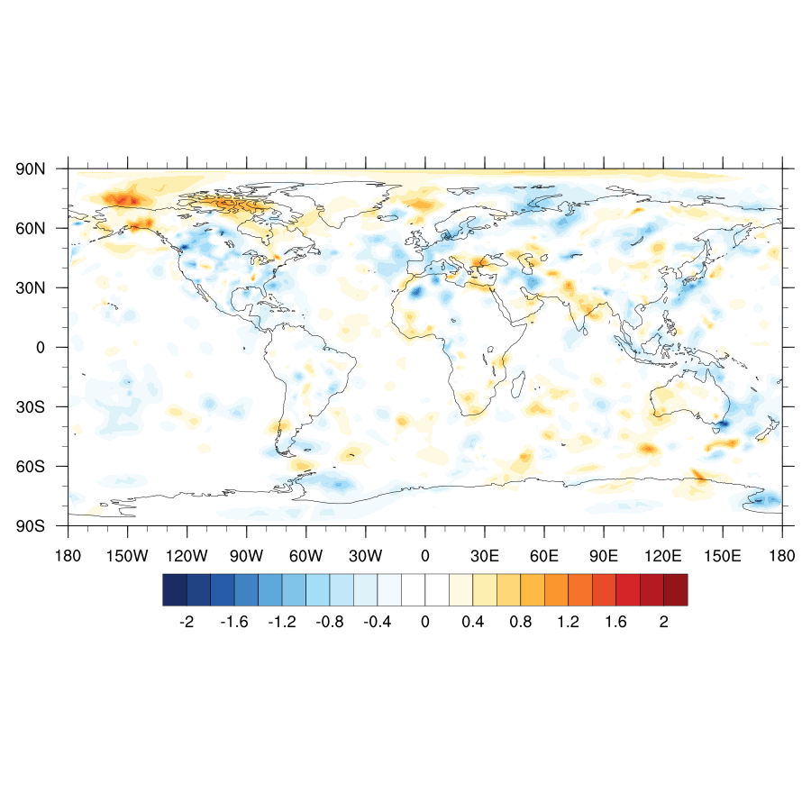
With the plot_eda_ens_spread.ncl, we can plot the ensemble spread of both background and analysis. Similar to the ensemble mean increments, just change the diag_var and diag_lev in the NCL script, and run plot_eda_ens_spread.ncl:

$ ncl plot_eda_ens_spread.ncl

This will produce a figure eda_ens_spread_surface_pressure_lev0.png.

We can also plot the vertical profiles of RMSE, BIAS, and total spread of the Innovations (Obs minus Bak) and Residuals (Obs minus Ana) with plot_eda_vert_profile_err.ncl. We need to specify the diag_obs, diag_var and nens (if run fewer EDA members) in the script:

diag_obs="sondes"
diag_var="windEastward"
nens = 10

Running:

$ ncl plot_eda_vert_profile_err.ncl

will produce a figure file eda_vert_profile_sondes_windEastward.png:

In this subsection, we will further run a single-time LETKF analysis. First, we need to create the working directory for LETKF and move to that directory:

$ mkdir -p /glade/derecho/scratch/$USER/mpas_jedi_tutorial/letkf
$ cd /glade/derecho/scratch/$USER/mpas_jedi_tutorial/letkf

Set environment variable for the mpas-bundle directory,

$ export bundle_dir=/glade/derecho/scratch/bjung/mpas_bundle_v4.0.1_public_prebuilt

Similar to EDA, we first prepare necessary files for LETKF.

$ ln -sf ../MPAS_namelist_stream_physics_files/*BL .
$ ln -sf ../MPAS_namelist_stream_physics_files/*DATA .
$ ln -sf ../MPAS_namelist_stream_physics_files/x1.10242.graph.info.part.64 .
$ ln -sf ../MPAS_namelist_stream_physics_files/streams.atmosphere_240km .
$ ln -sf ../MPAS_namelist_stream_physics_files/stream_list.atmosphere.* .
$ ln -sf ../MPAS_namelist_stream_physics_files/namelist.atmosphere_240km .
$ ln -sf ../MPAS_namelist_stream_physics_files/x1.10242.invariant.nc .
$ ln -sf ../background/2018041418/mpasout.2018-04-15_00.00.00.nc ./templateFields.10242.nc
$ ln -sf ${bundle_dir}/code/mpas-jedi/test/testinput/namelists/geovars.yaml  ./
$ ln -sf ${bundle_dir}/code/mpas-jedi/test/testinput/namelists/keptvars.yaml  ./
$ ln -sf ${bundle_dir}/code/mpas-jedi/test/testinput/obsop_name_map.yaml ./

Now prepare 'bg' and 'an' folders under letkf.

$ cp ../eda/prep_an_bg_directories.csh .
$ ./prep_an_bg_directories.csh
$ cp -r an/mem001 an/mem000

The reason of creating an/mem000 is that LETKF also writes out the mean of ensemble analyses under an/mem000. For observation-related directories, we need to create dbIn, dbOut, and dbAna directories, and link IODA observation files to dbIn directory:

$ mkdir dbIn dbOut dbAna
$ cd dbIn
$ ln -sf ../../obs_ioda/2018041500/aircraft_obs_2018041500.h5  ./
$ ln -sf ../../obs_ioda/2018041500/gnssro_obs_2018041500.h5    ./
$ ln -sf ../../obs_ioda/2018041500/sfc_obs_2018041500.h5       ./
$ ln -sf ../../obs_ioda/2018041500/satwind_obs_2018041500.h5   ./
$ ln -sf ../../obs_ioda/2018041500/sondes_obs_2018041500.h5    ./
$ cd ..

link the yaml files and scripts for LETKF:

$ ln -sf ../MPAS_JEDI_yamls_scripts/letkf_observer.yaml ./
$ ln -sf ../MPAS_JEDI_yamls_scripts/letkf_solver.yaml ./
$ ln -sf ../MPAS_JEDI_yamls_scripts/letkf_solver_vloc.yaml ./
$ ln -sf ../MPAS_JEDI_yamls_scripts/letkf_diagoma.yaml ./
$ ln -sf ../MPAS_JEDI_yamls_scripts/run_letkf_observer.csh ./
$ ln -sf ../MPAS_JEDI_yamls_scripts/run_letkf_solver.csh ./
$ ln -sf ../MPAS_JEDI_yamls_scripts/run_letkf_diagoma.csh ./

letkf_observer.yaml, letkf_solver.yaml, and letkf_diagoma.yaml are used for the three steps of LETKF. letkf_observer.yaml is for calculating the ensemble HofX of background and performing quality control based on the ensemble mean. letkf_solver.yaml is for updating the ensemble mean and ensemble members. letkf_diagoma.yaml is for calculating the ensemble HofX of analysis for OMA diagnosis.

We first submit run_letkf_observer.csh:

$ qsub run_letkf_observer.csh

This observer step will produce obsout_da_*.h5 files in dbOut. In each hdf5 file, we can see groups of hofx_0_*, hofx_y_mean_xb0, ombg, EffectiveQC0, EffectiveError0.

Then, submit run_letkf_solver.csh:

$ qsub run_letkf_solver.csh

This solver step will update an/mem*/an.2018-04-15_00.00.00.nc files, including the ensemble mean of analysis an/mem000/an.2018-04-15_00.00.00.nc.

Last, submit run_letkf_diagoma.csh:

$ qsub run_letkf_diagoma.csh

The analysis-diagnostic step will generate obsout_*.h5 files in dbAna, similar to the files in dbOut but for HofX of ensemble analysis.

The previous run only tests the horizontal localization. If we want to also employ the vertical localization, just change

_height-based obs localizations: &heightAndHorizObsLoc
  <<: *2DLETKFheightAndHorizObsLoc

to

_height-based obs localizations: &heightAndHorizObsLoc
  <<: *3DLETKFheightAndHorizObsLoc

in letkf_solver.yaml, and then resubmit run_letkf_solver.csh and run_letkf_diagoma.csh. Backup an and dbAna directories before another run.

Similar to the EDA test, we also prepared some NCL scripts to plot LETKF results.

$ cp ../ncl_scripts/plot_letkf_*.ncl .

Plotting the analysis increment of ensemble mean with plot_letkf_ensmean_anainc.ncl. We need to specify the diag_var and diag_lev (for 3-D variables) in the NCL script.

    diag_var="surface_pressure"
    diag_lev=10

Then do:

$ ncl plot_letkf_ensmean_anainc.ncl

This will produce a figure letkf_ens_mean_inc_surface_pressure_lev0.png.

For plotting ensemble spread of both background and analysis, you could change diag_var and diag_lev in plot_letkf_ens_spread.ncl before running:

$ ncl plot_letkf_ens_spread.ncl

This will produce a figure letkf_ens_spread_surface_pressure_lev0.png.

For plotting the vertical profiles of RMSE, BIAS, and total spread of the Innovations (Obs minus Bak) and Residuals (Obs minus Ana) with plot_letkf_vert_profile_err.ncl, we could specify the diag_obs and diag_var in the script:

diag_obs="sondes"
diag_var="windEastward"

then run:

$ ncl plot_letkf_vert_profile_err.ncl

This will produce a figure letkf_vert_profile_sondes_windEastward.png.