This web page is intended to serve as a guide through the practice exercises of this
tutorial. Exercises are split into seven main sections, each of which focuses on
a particular aspect of using the MPAS-Atmosphere model.
While going through this practice guide, you may find it helpful to have a copy
of the MPAS-Atmosphere Users' Guide available in another window.
Click here
to open the Users' Guide in a new window.
In case you would like to refer to any of the lecture slides from previous days,
you can open the Tutorial Agenda in another window.
You can proceed through the sections of this practical guide at your own pace. It is highly recommended
to go through the exercises in order, since later exercises may require the output of earlier ones.
Clicking the grey headers will expand each section or subsection.
The practical exercises in this tutorial have been tailored to work on
the Cheyenne system.
Cheyenne is an HPC cluster that provides most of the libraries needed by MPAS and its pre- and post-processing
tools through modules. In general, before compiling and running MPAS-Atmosphere on your own system,
you will need an MPI-2 implementation as well as the NetCDF-4, PnetCDF, and PIO libraries.
Beginning with MPAS v8.0, a built-in alternative to the PIO library is available: the Simple MPAS
I/O Layer (SMIOL). SMIOL requires just the PnetCDF library, and there is no need for the NetCDF-4
and PIO libraries when compiling MPAS itself. In this tutorial, we will be using MPAS with the SMIOL
library.
Before going through any of the exercises in subsequent sections, we will need to run
several commands to prepare our environment. Firstly, we will purge all loaded modules to begin
from a known starting point (with no modules loaded); then, we will load several modules to give
access to the GNU compilers as well as an MPI implementation:
$ module purge
$ module load ncarenv/1.3
$ module load gnu/10.1.0
$ module load ncarcompilers/0.5.0
$ module load mpt/2.25
Next, we will load modules for additional libraries needed by the MPAS-Atmosphere model.
Besides the Parallel-NetCDF module (pnetcdf/1.12.2) needed
by MPAS itself, the netcdf-mpi/4.8.1 module is being loaded
to support compilation of pre- and post-processing tools and so that we have access to
the standard ncdump program for showing the contents
of NetCDF files.
$ module load pnetcdf/1.12.2
$ module load netcdf-mpi/4.8.1
At this point, running module list should print the following:
$ module list

Currently Loaded Modules:
  1) ncarenv/1.3   3) ncarcompilers/0.5.0   5) pnetcdf/1.12.2
  2) gnu/10.1.0    4) mpt/2.25              6) netcdf-mpi/4.8.1
Post-processing exercises will need Python along with the NumPy, PyNGL, NetCDF4,
and miscellaneous other Python packages. On Cheyenne, these are available in
a Conda environment named 'npl'. The npl environment also provides the NCAR Command
Language (NCL). We can load the conda module and activate the npl environment with
the following commands:
$ module load conda
$ conda activate npl
Some Python plotting scripts that will be used in this tutorial rely on
additional Python code that is located in a non-standard location.
In order for these plotting scripts to work, we'll need to set our
PYTHONPATH environment variable using the following command:
$ export PYTHONPATH=/glade/p/mmm/wmr/mpas_tutorial/python_scripts
Additionally, we can load a module to provide access to the 'ncview' tool:
$ module load ncview
When running limited-area simulations, we will need to use Metis to create
our own graph partition files. We can add the gpmetis command
to our PATH with the following:
$ export PATH=/glade/p/mmm/wmr/mpas_tutorial/metis-5.1.0-gcc9.1.0/bin:${PATH}
IMPORTANT NOTE:The 'npl' Conda environment on Cheyenne modifies
our PATH such that the wrong MPI compiler wrappers appear
first. To remedy this, we can simply reload the 'gnu' module as a final step:
$ module reload gnu
If you've logged out of Cheyenne and would like a quick list of commands to set up your
environment again after logging back in, you can copy and paste the following commands
into your terminal:
module purge
module load ncarenv/1.3
module load gnu/10.1.0
module load ncarcompilers/0.5.0
module load mpt/2.25
module load pnetcdf/1.12.2
module load netcdf-mpi/4.8.1
module load conda
conda activate npl
export PYTHONPATH=/glade/p/mmm/wmr/mpas_tutorial/python_scripts
module load ncview
export PATH=/glade/p/mmm/wmr/mpas_tutorial/metis-5.1.0-gcc9.1.0/bin:${PATH}
module reload gnu
We will run all of the practical exercises in this tutorial in our scratch directories,
i.e., /glade/scratch/$USER. To keep the MPAS tutorial exercises separate
from other work, we'll create a sub-directory named "mpas_tutorial":
$ mkdir /glade/scratch/$USER/mpas_tutorial
Running jobs on Cheyenne requires the submission of a job script to a batch queueing system,
which will allocate requested computing resources to your job when they become available.
In general, it's best to avoid running any compute-intensive jobs on the login nodes, and
the practical instructions to follow will guide you in the process of submitting jobs when
necessary.
As a first introduction to running jobs on Cheyenne, there are several key commands worth
noting:
- qcmd -A UMMM0004 - This command runs the specified command on a batch node under
the UMMM0004 project for this tutorial
- qsub - This command submits a job script, which describes a job
to be run on one or more batch nodes; it offers increased
control over running a simple command with qcmd
- qstat -u $USER - This command tells you the status of your pending and running jobs.
Note that you may need to wait about 30 seconds for a recently submitted job to show up.
- qdel - This command deletes a queued or running job
At various points in the practical exercises, we'll need to submit jobs to Cheyenne's queueing system
using the qsub command, and after doing so, we may often check on the status
of the job with the qstat command, monitoring the log files produced by the job
once we see that the job has begun to run.
With your shell environment set up as described in this section, you're ready to begin with the
practical exercises of this tutorial!
In this section, our goal is to obtain a copy of the MPAS source code directly from the MPAS
GitHub repository. We'll then compile both the init_atmosphere_model
and atmosphere_model programs before using the former to begin
the processing of time-invariant, terrestrial fields for use in a real-data simulation. While
this processing is taking place, in another terminal window
(don't forget to set up your environment!)
we can practice preparing idealized initial conditions.
Since our default login shell is bash, all shell commands
throughout this tutorial will be written for bash. However, if you prefer a different
shell and don't mind mentally translating, e.g., export commands to
setenv commands, then feel free to switch shells.
As described in the lectures, the MPAS code is distributed directly from the GitHub
repository where it is developed. While it's possible to navigate to
https://github.com/MPAS-Dev/MPAS-Model
and obtain the code by clicking on the "Releases" tab, it's much faster to clone
the repository directly on the command-line. After changing to our /glade/scratch/${USER}/mpas_tutorial directory, we can
make a clone of the MPAS-Model repository:
$ cd /glade/scratch/${USER}/mpas_tutorial
$ git clone https://github.com/MPAS-Dev/MPAS-Model.git
Cloning the MPAS-Model repository may take a few seconds, and at the end of the process,
the output to the terminal should look something like the following:
Cloning into 'MPAS-Model'...
remote: Enumerating objects: 64819, done.
remote: Counting objects: 100% (29/29), done.
remote: Compressing objects: 100% (13/13), done.
remote: Total 64819 (delta 16), reused 25 (delta 16), pack-reused 64790
Receiving objects: 100% (64819/64819), 35.63 MiB | 20.78 MiB/s, done.
Resolving deltas: 100% (48230/48230), done.
Updating files: 100% (1540/1540), done.
We should now have an MPAS-Model directory:
$ ls -l MPAS-Model
total 36
-rw-r--r--  1 duda ncar  3131 Apr  7 21:01 INSTALL
-rw-r--r--  1 duda ncar  2311 Apr  7 21:01 LICENSE
-rw-r--r--  1 duda ncar 27607 Apr  7 21:01 Makefile
-rw-r--r--  1 duda ncar  2555 Apr  7 21:01 README.md
drwxr-xr-x 14 duda ncar  4096 Apr  7 21:01 src
drwxr-xr-x  4 duda ncar  4096 Apr  7 21:01 testing_and_setup
That's it! We now have a copy of the latest release of the MPAS source code.
As mentioned in the lectures, there are two "cores" that need to be compiled from
the same MPAS source code: the init_atmosphere core and
the atmosphere core.
Before beginning the compilation process, it's worth verifying that we have
MPI compiler wrappers in our path, and that environment variable pointing to
the Parallel-NetCDF library is set:
$ which mpif90
/glade/u/apps/ch/opt/ncarcompilers/0.5.0/gnu/10.1.0/mpi/mpif90

$ which mpicc
/glade/u/apps/ch/opt/ncarcompilers/0.5.0/gnu/10.1.0/mpi/mpicc

$ echo $PNETCDF
/glade/u/apps/ch/opt/pnetcdf/1.12.2/mpt/2.25/gnu/10.1.0/
If all of the above commands were successful, our shell environment should be
sufficient to allow the MPAS cores to be compiled.
We'll begin by compiling the init_atmosphere core, producing an executable
named init_atmosphere_model.
IMPORTANT NOTE:Before compiling on Cheyenne specifically, there's an important point that needs explanation!
In order to avoid saturating the Cheyenne login nodes with compilation processes and negatively impacting other
users, we will run our compilation command on a batch node with the special qcmd command.
The qcmd command launches the specified command on a batch node and returns when the command
has finished. So, although you would normally not use "qcmd" when compiling MPAS on other systems, for this tutorial
we will prefix the usual compilation command with qcmd -A UMMM0004 -- (where UMMM0004 is
the computing project we're working under).
After changing to the MPAS-Model directory
$ cd MPAS-Model
we can issue the following command to build the init_atmosphere core with
the gfortran compiler:
$ qcmd -A UMMM0004 -- make -j4 gfortran CORE=init_atmosphere PRECISION=single
Note the inclusion of PRECISION=single on the build command;
the default is to build MPAS cores as double-precision executables, but single-precision
executables require less memory, produce smaller output files, run faster, and — at least
for MPAS-Atmosphere — seem to produce results that are no worse than double-precision executables.
In the build command, we have also added the -j4 flag to tell make
to use four tasks to build the code; this should reduce the time to compile the init_atmosphere_model
executable significantly!
After issuing the make command, above, compilation should take just a couple of
minutes, and if the compilation was successful, the end of the build process should have produced
messages like the following:
*******************************************************************************
MPAS was built with default single-precision reals.
Debugging is off.
Parallel version is on.
Papi libraries are off.
TAU Hooks are off.
MPAS was built without OpenMP support.
MPAS was built with .F files.
The native timer interface is being used
Using the SMIOL library.
*******************************************************************************
If compilation of the init_atmosphere core was successful, we should also have an executable
file named init_atmosphere_model:
$ ls -l
total 2006
drwxr-xr-x  2 duda ncar    4096 Apr 26 20:32 default_inputs
-rwxr-xr-x  1 duda ncar 2014592 Apr 26 20:32 init_atmosphere_model
-rw-r--r--  1 duda ncar    3131 Apr 26 20:26 INSTALL
-rw-r--r--  1 duda ncar    2311 Apr 26 20:26 LICENSE
-rw-r--r--  1 duda ncar   27864 Apr 26 20:26 Makefile
-rw-r--r--  1 duda ncar    1379 Apr 26 20:32 namelist.init_atmosphere
-rw-r--r--  1 duda ncar    2555 Apr 26 20:26 README.md
drwxr-xr-x 14 duda ncar    4096 Apr 26 20:32 src
-rw-r--r--  1 duda ncar     920 Apr 26 20:32 streams.init_atmosphere
drwxr-xr-x  4 duda ncar    4096 Apr 26 20:26 testing_and_setup
Note, also, that default namelist and streams files for the init_atmosphere core
have also been generated as part of the compilation process: these are the files named
namelist.init_atmosphere and streams.init_atmosphere.
Now, we're ready to compile the atmosphere core. If we try this without cleaning any
of the common infrastructure code, first, e.g.,
$ make gfortran CORE=atmosphere PRECISION=single
we would get an error like the following:
*******************************************************************************
 The MPAS infrastructure is currently built for the init_atmosphere_model core.
 Before building the atmosphere core, please do one of the following.


 To remove the init_atmosphere_model_model executable and clean the MPAS infrastructure, run:
      make clean CORE=init_atmosphere_model

 To preserve all executables except atmosphere_model and clean the MPAS infrastructure, run:
      make clean CORE=atmosphere

 Alternatively, AUTOCLEAN=true can be appended to the make command to force a clean,
 build a new atmosphere_model executable, and preserve all other executables.

*******************************************************************************
After compiling one MPAS core, we need to clean up the shared infrastructure before
compiling a different core. We can clean all parts of the infrastructure that are
needed by the atmosphere core by running the following command:
$ make clean CORE=atmosphere
IMPORTANT NOTE:Because we are compiling on the batch nodes of Cheyenne, and because the batch
nodes do not have internet access, we need to manually obtain lookup tables used by physics schemes when compiling
on Cheyenne with qcmd. In general, the next step is not needed when compiling on, e.g., login nodes that have
internet access.
Before launching the model compilation on a batch node with qcmd, we can manually obtain physics lookup tables
with the following commands from our top-level MPAS-Model directory:
$ cd src/core_atmosphere/physics
$ ./checkout_data_files.sh
$ cd ../../..
Having manually obtain physics lookup tables, we can proceed to compile the atmosphere
core in single-precision with:
$ qcmd -A UMMM0004 -- make -j4 gfortran CORE=atmosphere PRECISION=single
The compilation of the atmosphere_model executable can take
several minutes or longer to complete (depending on which compiler is used).
Similar to the compilation of the init_atmosphere core, a successful compilation
of the atmosphere core should give the following message:
*******************************************************************************
MPAS was built with default single-precision reals.
Debugging is off.
Parallel version is on.
Papi libraries are off.
TAU Hooks are off.
MPAS was built without OpenMP support.
MPAS was built with .F files.
The native timer interface is being used
Using the SMIOL library.
*******************************************************************************
Now, our MPAS-Model directory should contain an executable file named atmosphere_model,
as well as default namelist.atmosphere and streams.atmosphere
files:
$ ls -lL
total 33018
-rwxr-xr-x  1 duda ncar  5644864 Apr 26 20:37 atmosphere_model
-rwxr-xr-x  1 duda ncar   209256 Apr 26 20:36 build_tables
-rw-r--r--  1 duda ncar 20580056 Apr 26 20:34 CAM_ABS_DATA.DBL
-rw-r--r--  1 duda ncar    18208 Apr 26 20:34 CAM_AEROPT_DATA.DBL
drwxr-xr-x  2 duda ncar     4096 Apr 26 20:37 default_inputs
-rw-r--r--  1 duda ncar      261 Apr 26 20:34 GENPARM.TBL
-rwxr-xr-x  1 duda ncar  2014592 Apr 26 20:32 init_atmosphere_model
-rw-r--r--  1 duda ncar     3131 Apr 26 20:26 INSTALL
-rw-r--r--  1 duda ncar    29820 Apr 26 20:34 LANDUSE.TBL
-rw-r--r--  1 duda ncar     2311 Apr 26 20:26 LICENSE
-rw-r--r--  1 duda ncar    27864 Apr 26 20:26 Makefile
-rw-r--r--  1 duda ncar     1774 Apr 26 20:37 namelist.atmosphere
-rw-r--r--  1 duda ncar     1379 Apr 26 20:32 namelist.init_atmosphere
-rw-r--r--  1 duda ncar   543744 Apr 26 20:34 OZONE_DAT.TBL
-rw-r--r--  1 duda ncar      536 Apr 26 20:34 OZONE_LAT.TBL
-rw-r--r--  1 duda ncar      708 Apr 26 20:34 OZONE_PLEV.TBL
-rw-r--r--  1 duda ncar     2555 Apr 26 20:26 README.md
-rw-r--r--  1 duda ncar   847552 Apr 26 20:34 RRTMG_LW_DATA
-rw-r--r--  1 duda ncar  1694976 Apr 26 20:34 RRTMG_LW_DATA.DBL
-rw-r--r--  1 duda ncar   680368 Apr 26 20:34 RRTMG_SW_DATA
-rw-r--r--  1 duda ncar  1360572 Apr 26 20:34 RRTMG_SW_DATA.DBL
-rw-r--r--  1 duda ncar     4399 Apr 26 20:34 SOILPARM.TBL
drwxr-xr-x 14 duda ncar     4096 Apr 26 20:37 src
-rw-r--r--  1 duda ncar     1203 Apr 26 20:37 stream_list.atmosphere.diagnostics
-rw-r--r--  1 duda ncar      927 Apr 26 20:37 stream_list.atmosphere.output
-rw-r--r--  1 duda ncar        9 Apr 26 20:37 stream_list.atmosphere.surface
-rw-r--r--  1 duda ncar     1571 Apr 26 20:37 streams.atmosphere
-rw-r--r--  1 duda ncar      920 Apr 26 20:32 streams.init_atmosphere
drwxr-xr-x  4 duda ncar     4096 Apr 26 20:26 testing_and_setup
-rw-r--r--  1 duda ncar    22986 Apr 26 20:34 VEGPARM.TBL
Note, also, the presence of files named stream_list.atmosphere.*. These are lists
of output fields that are referenced by the streams.atmosphere file.
The new files like CAM_ABS_DATA.DBL, LANDUSE.TBL, RRTMG_LW_DATA, etc. are look-up tables and other data files used by physics schemes in MPAS-Atmosphere. These files
should all be symbolic links to files in the src/core_atmosphere/physics/physics_wrf/files/ directory.
If we have init_atmosphere_model and atmosphere_model
executables, then compilation of both MPAS-Atmosphere cores was successful, and we're ready to proceed
to the next sub-section.
For our first MPAS simulation in this tutorial, we'll use a quasi-uniform 240-km mesh. Since
we'll later be working with a variable-resolution mesh, it will be helpful to maintain separate
sub-directories for these two simulations.
To begin processing of the static, terrestrial fields for the 240-km quasi-uniform mesh, let's
change to our /glade/scratch/${USER}/mpas_tutorial directory and make a new sub-directory named 240km_uniform:
$ cd /glade/scratch/${USER}/mpas_tutorial
$ mkdir 240km_uniform
$ cd 240km_uniform
We can find a copy of the 240-km quasi-uniform mesh at /glade/p/mmm/wmr/mpas_tutorial/meshes/x1.10242.grid.nc.
To save disk space, we'll symbolically link this file into our directory:
$ ln -s /glade/p/mmm/wmr/mpas_tutorial/meshes/x1.10242.grid.nc .
We will also need the init_atmosphere_model executable, as well as copies
of the namelist.init_atmosphere and streams.init_atmosphere
files. We'll make a symbolic link to the executable, and copies of the other files (since we will be changing them):
$ ln -s /glade/scratch/${USER}/mpas_tutorial/MPAS-Model/init_atmosphere_model .
$ cp /glade/scratch/${USER}/mpas_tutorial/MPAS-Model/namelist.init_atmosphere .
$ cp /glade/scratch/${USER}/mpas_tutorial/MPAS-Model/streams.init_atmosphere .
Before running the init_atmosphere_model program, we'll need to set
up the namelist.init_atmosphere file as described in the lectures.
With your preferred editor, edit the highlighted options in the default
namelist.init_atmosphere file so that they match the following:
&nhyd_model
    config_init_case = 7
/
&data_sources
    config_geog_data_path = '/glade/p/mmm/wmr/mpas_tutorial/mpas_static/'
    config_landuse_data = 'MODIFIED_IGBP_MODIS_NOAH'
    config_topo_data = 'GMTED2010'
    config_vegfrac_data = 'MODIS'
    config_albedo_data = 'MODIS'
    config_maxsnowalbedo_data = 'MODIS'
    config_supersample_factor = 3
/
&preproc_stages
    config_static_interp = true
    config_native_gwd_static = true
    config_vertical_grid = false
    config_met_interp = false
    config_input_sst = false
    config_frac_seaice = false
/
Note, in particular, the setting of the path to the geographical data sets, and the
settings to enable only the processing of static data and the gravity wave drag ("gwd")
static fields.
After editing the namelist.init_atmosphere file, it will also be necessary to tell the
init_atmosphere_model program the name of our input grid file, as well as the name of the
"static" output file that we would like to create. We do this by editing the streams.init_atmosphere
file, where we first set the name of the grid file for the "input" stream:
<immutable_stream name="input"
                  type="input"
                  filename_template="x1.10242.grid.nc"
                  input_interval="initial_only"/>
and then set the name of the static file to be created for the "output" stream:
<immutable_stream name="output"
                  type="output"
                  filename_template="x1.10242.static.nc"
                  packages="initial_conds"
                  output_interval="initial_only" />
When interpolating geographical fields to a mesh, the "surface" and "lbc" streams can be ignored (but, you should
not delete the "surface" or "lbc" streams, or the init_atmosphere_model program will complain).
After editing the streams.init_atmosphere file, we can begin the processing
of the static, time-invariant fields for the 240-km quasi-uniform mesh.
Rather than running the init_atmosphere_model program on a batch node with
qcmd, we will use a job script to run the program, returning a command prompt
to us where we can monitor the progress of the job. To begin, we'll copy a prepared job script to our
working directory:
$ cp /glade/p/mmm/wmr/mpas_tutorial/job_scripts/init_real.pbs .
If you're interested in doing so, you can take a look at the init_real.pbs job script.
Once you're ready, you can submit the script to the queueing system with the qsub command:
$ qsub init_real.pbs
Now, we need to wait for our job to start running; we can check on its status every minute or so with
the qstat command:
$ qstat -u $USER
Once we see that our job is running — indicated by an "R" in the second-to-last column, e.g,
$ qstat -u $USER

chadmin1.ib0.cheyenne.ucar.edu:
                                                            Req'd  Req'd   Elap
Job ID          Username Queue    Jobname    SessID NDS TSK Memory Time  S Time
--------------- -------- -------- ---------- ------ --- --- ------ ----- - -----
7497852.chadmin duda     regular  240km_stat  25299   1   1    --  02:00 R 00:00
we can check on the progress of the init_atmosphere_model program
by following the messages written to the log.init_atmosphere.0000.out
file:
$ tail -f log.init_atmosphere.0000.out
We should expect to see lines of output similar to the following being printed every few seconds:
 /glade/p/mmm/wmr/mpas_tutorial/mpas_static/topo_gmted2010_30s/28801-30000.03601-04800
 /glade/p/mmm/wmr/mpas_tutorial/mpas_static/topo_gmted2010_30s/30001-31200.03601-04800
 /glade/p/mmm/wmr/mpas_tutorial/mpas_static/topo_gmted2010_30s/31201-32400.03601-04800
 /glade/p/mmm/wmr/mpas_tutorial/mpas_static/topo_gmted2010_30s/32401-33600.03601-04800
 /glade/p/mmm/wmr/mpas_tutorial/mpas_static/topo_gmted2010_30s/33601-34800.03601-04800
 /glade/p/mmm/wmr/mpas_tutorial/mpas_static/topo_gmted2010_30s/34801-36000.03601-04800
 /glade/p/mmm/wmr/mpas_tutorial/mpas_static/topo_gmted2010_30s/36001-37200.03601-04800
 /glade/p/mmm/wmr/mpas_tutorial/mpas_static/topo_gmted2010_30s/37201-38400.03601-04800
 /glade/p/mmm/wmr/mpas_tutorial/mpas_static/topo_gmted2010_30s/38401-39600.03601-04800
 /glade/p/mmm/wmr/mpas_tutorial/mpas_static/topo_gmted2010_30s/39601-40800.03601-04800
 /glade/p/mmm/wmr/mpas_tutorial/mpas_static/topo_gmted2010_30s/40801-42000.03601-04800
 /glade/p/mmm/wmr/mpas_tutorial/mpas_static/topo_gmted2010_30s/42001-43200.03601-04800
 /glade/p/mmm/wmr/mpas_tutorial/mpas_static/topo_gmted2010_30s/00001-01200.04801-06000
 /glade/p/mmm/wmr/mpas_tutorial/mpas_static/topo_gmted2010_30s/01201-02400.04801-06000
 /glade/p/mmm/wmr/mpas_tutorial/mpas_static/topo_gmted2010_30s/02401-03600.04801-06000
 /glade/p/mmm/wmr/mpas_tutorial/mpas_static/topo_gmted2010_30s/03601-04800.04801-06000
The processing of the static, time-invariant fields will take some time — perhaps 30 – 45 minutes or so.
If lines similar to the above are being periodically written, we can kill the tail
process with CTRL-C before proceeding to the next sub-section, where we will create
idealized initial conditions while the static, terrestrial fields are interpolated.
IMPORTANT NOTE: If lines of output are not being periodically written to the terminal
when running the tail command as described above, look for a file
named log.init_atmosphere.0000.err and detemine what went wrong before
going on to the next sub-section! Exercises in the second section of this tutorial will require
the successful processing of static, time-invariant fields!
While the init_atmosphere_model program is processing static,
time-invariant fields for a real-data simulation in the 240km_uniform
directory, we can try initializing and running an idealized simulation in a separate directory.
The init_atmosphere_model program supports the creation of idealized
initial conditions for the following cases:
- 3-d baroclinic wave on the sphere
- 3-d supercell thunderstorm on a doubly-periodic Cartesian plane
- 2-d mountain wave in the xz-plane
For each of these idealized cases, prepared input files are available on the MPAS-Atmosphere
download page. We'll go through the process of creating initial conditions for the idealized
supercell case; the general process is similar for the other two cases.
The prepared input files for MPAS-Atmosphere idealized cases may be found by going to
the MPAS Homepage and clicking
on the "MPAS-Atmosphere download" link at the left. Then, clicking on the "Configurations
for idealized test cases" link will take you to the download links for idealized cases.
Although the input files for these idealized cases can be downloaded through the web page,
we can also download, e.g., the supercell input files with wget
once we know the URL. Beginning from our /glade/scratch/${USER}/mpas_tutorial directory, we can download the supercell
input file archive and unpack it with:
$ cd /glade/scratch/${USER}/mpas_tutorial
$ wget http://www2.mmm.ucar.edu/projects/mpas/test_cases/v7.0/supercell.tar.gz
$ tar xzvf supercell.tar.gz
After changing to the resulting supercell directory,
the README file will give an overview of how to initialize and
run the test case. The key points are that we need to symbolically link both
the init_atmosphere_model and atmosphere_model
executables into the supercell directory:
$ ln -s /glade/scratch/${USER}/mpas_tutorial/MPAS-Model/init_atmosphere_model .
$ ln -s /glade/scratch/${USER}/mpas_tutorial/MPAS-Model/atmosphere_model .
Unlike as described in the README file, however, we will not run
the init_atmosphere_model and atmosphere_model
programs directly on the command-line.
We will run the init_atmosphere_model program through qcmd with:
$ qcmd -A UMMM0004 -- ./init_atmosphere_model
Once the initial conditions have been created as described in the README
file, it's helpful to verify that there were no errors; the end of
the log.init_atmosphere.0000.out
file should look something like the following:
 -----------------------------------------
 Total log messages printed:
    Output messages =                  304
    Warning messages =                  13
    Error messages =                     0
    Critical error messages =            0
 -----------------------------------------
Assuming there were no errors, we can run the simulation with 32 processors by first copying
a prepared job script to our working directory and submitting the script with qsub:
$ cp /glade/p/mmm/wmr/mpas_tutorial/job_scripts/supercell.pbs .
$ qsub supercell.pbs
As with the static field interpolation, we need to wait for our job to start running. We can check on its
status every minute or so with the qstat command:
$ qstat -u $USER
Once we see that our job is running, we can move on to the next section.
The simulation may take about 10 minutes to run with 32 MPI tasks. During one of the later
practical section, if you would like to revisit the simulation to see the results, running
the supercell.ncl NCL script should produce plots
of the time evolution of several model fields:
$ ncl supercell.ncl
Having compiled both the init_atmosphere and atmosphere
cores, and also having interpolated time-invariant, terrestrial fields to create a "static" file for
real-data simulations, we'll interpolate atmospheric and land-surface fields to create complete initial
conditions for an MPAS simulation in this section. We'll also process 10 days' worth of SST and sea-ice
data to update these fields periodically as the model runs. Then, we'll start a five-day simulation,
which will take around an hour to complete. Once the model has started running, we can use any extra time
to compile the convert_mpas utility program.
If you've reached this point and the static field interpolation from Section 1.3 has not yet
finished, you can first go through Section 2.4, before returning to Sections 2.1 - 2.3 after
the static field interpolation has completed.
In an earlier section, we started the process of interpolating static geographical
fields to the 240-km, quasi-uniform mesh in the 240km_uniform
directory. If this interpolation was successful, this directory should contain two new
files: log.init_atmosphere.0000.out and
x1.10242.static.nc.
$ cd /glade/scratch/${USER}/mpas_tutorial/240km_uniform
$ ls -l log.init_atmosphere.0000.out x1.10242.static.nc
The end of the log.init_atmosphere.0000.out file should show
that there were no errors:
 -----------------------------------------
 Total log messages printed:
    Output messages =                 2915
    Warning messages =                  10
    Error messages =                     0
    Critical error messages =            0
 -----------------------------------------
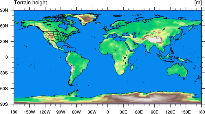
We can also make a plot of the terrain elevation field in the x1.10242.static.nc
file with a Python script named plot_terrain.py. We'll discuss the use of Python
and NCL scripts for visualization in a later section, so for now we can simply execute the following
commands to plot the terrain field:
$ cp /glade/p/mmm/wmr/mpas_tutorial/python_scripts/plot_terrain.py .
$ ./plot_terrain.py x1.10242.static.nc
$ display terrain.png
Running the script may take 10 or 15 seconds, but the result should be a figure that looks
like the following:
Now that we have convinced ourselves that the processing of static, geographical fields was successful,
we can proceed to interpolate atmosphere and land-surface initial conditions for our 240-km simulation.
Generally, it is necessary to use the ungrib component of the WRF Pre-Processing System to prepare
atmospheric datasets in the intermediate format used by MPAS. For the purposes of this tutorial,
we will simply assume that these data have already been processed with the ungrib program in
/glade/p/mmm/wmr/mpas_tutorial/met_data/.
To interpolate the ERA5 analysis valid at 0000 UTC on 10 September 2014 to our 240-km mesh, we will
symbolically link the ERA5:2014-09-10_00 file to our working directory:
$ ln -s /glade/p/mmm/wmr/mpas_tutorial/met_data/ERA5:2014-09-10_00 .
Then, we will need to edit the namelist.init_atmosphere as described in the lectures
to instruct the init_atmosphere_model program to interpolate the ERA5 data to our mesh.
The critical items to set in the namelist.init_atmosphere file are:
&nhyd_model
    config_init_case = 7
    config_start_time = '2014-09-10_00:00:00'
/
&dimensions
    config_nvertlevels = 41
    config_nsoillevels = 4
    config_nfglevels = 38
    config_nfgsoillevels = 4
/
&data_sources
    config_met_prefix = 'ERA5'
    config_use_spechumd = false
/
&vertical_grid
    config_ztop = 30000.0
    config_nsmterrain = 1
    config_smooth_surfaces = true
    config_dzmin = 0.3
    config_nsm = 30
    config_tc_vertical_grid = true
    config_blend_bdy_terrain = false
/
&interpolation_control
    config_extrap_airtemp = 'lapse-rate'
/
&preproc_stages
    config_static_interp = false
    config_native_gwd_static = false
    config_vertical_grid = true
    config_met_interp = true
    config_input_sst = false
    config_frac_seaice = true
/
You may find it easier to copy the default namelist.init_atmosphere file from
/glade/scratch/${USER}/mpas_tutorial/MPAS-Model/namelist.init_atmosphere before making the edits highlighted
above.
When editing the namelist.init_atmosphere file, the key changes are to
the starting time for our real-data simulation, the prefix of the intermediate file that
contains the ERA5 atmospheric and land-surface fields, and the pre-processing stages that will be run.
For this simulation, we'll also use just 41 vertical layers in the atmosphere, rather than the default
of 55, so that the simulation will run faster.
After editing the namelist.init_atmosphere file, we will also need to set
the name of the input file in the streams.init_atmosphere file to
the name of the "static" file that we just produced:
<immutable_stream name="input"
                  type="input"
                  filename_template="x1.10242.static.nc"
                  input_interval="initial_only"/>
and we will also need to set the name of the output file, which will be the MPAS real-data initial
conditions file:
<immutable_stream name="output"
                  type="output"
                  filename_template="x1.10242.init.nc"
                  packages="initial_conds"
                  output_interval="initial_only" />
Once we've made the above changes to the namelist.init_atmosphere and
streams.init_atmosphere files, we can run the init_atmosphere_model
program by submitting our init_real.pbs script again:
$ qsub init_real.pbs
As before, we can check on the status of our job periodically by running
$ qstat -u $USER
After it begins to run, the program should take just a minute or two to finish running, and the result should be
an x1.10242.init.nc file and a new log.init_atmosphere.0000.out
file. Assuming no errors were reported at the end of the log.init_atmosphere.0000.out file,
we can plot, e.g., the skin temperature field in the x1.10242.init.nc file using
the plot_tsk.py Python script:
$ cp /glade/p/mmm/wmr/mpas_tutorial/python_scripts/plot_tsk.py .
$ ./plot_tsk.py x1.10242.init.nc
$ display tsk.png
Again, we'll examine the use of Python and NCL scripts for visualization later, so for now we only need
to verify that a plot like the following is produced:
If a plot like the above is produced, then we have completed the generation of an initial conditions file for our
240-km real-data simulation!
Because MPAS-Atmosphere — at least, when run as a stand-alone model — does not
contain prognostic equations for the SST and sea-ice fraction, these fields would remain
constant if not updated from an external source; this is, of course, not realistic, and it
will generally impact the quality of longer model simulations. Consequently, for MPAS-Atmosphere
simulations longer than roughly a week, it is typically necessary
to periodically update the sea-surface temperature (SST) field in the model. For real-time
simulations, this is generally not an option, but it is feasible for retrospective
simulations, where we have observed SST analyses available to us.
In order to create an SST update file, we will make use of
a sequence of intermediate files containing SST and sea-ice analyses that are available
in /glade/p/mmm/wmr/mpas_tutorial/met_data. Before proceeding, we'll link all of these SST intermediate
files into our working directory:
$ ln -sf /glade/p/mmm/wmr/mpas_tutorial/met_data/SST* .
Following Section 8.1 of the MPAS-Atmosphere Users' Guide, we must edit the namelist.init_atmosphere
file to specify the range of dates for which we have SST data, as well as the frequency at which the SST
intermediate files are available. The key namelist options that must be set are shown below;
other options can be ignored.
&nhyd_model
    config_init_case = 8
    config_start_time = '2014-09-10_00:00:00'
    config_stop_time = '2014-09-20_00:00:00'
/

&data_sources
    config_sfc_prefix = 'SST'
    config_fg_interval = 86400
/

&preproc_stages
    config_static_interp = false
    config_native_gwd_static = false
    config_vertical_grid = false
    config_met_interp = false
    config_input_sst = true
    config_frac_seaice = true
/
Note in particular that we have set the config_init_case variable to 8! This is
the initialization case used to create surface update files, instead of real-data initial
conditions files.
As before, we also need to edit the streams.init_atmosphere file, this time setting the
name of the SST update file to be created by the "surface" stream, as well as the frequency
at which this update file should contain records:
<immutable_stream name="surface"
                  type="output"
                  filename_template="x1.10242.sfc_update.nc"
                  filename_interval="none"
                  packages="sfc_update"
                  output_interval="86400"/>
Note that we have set both the filename_template and output_interval attributes
of the "surface" stream. The output_interval should match the interval specified in the namelist
for the config_fg_interval variable. The other streams ("input", "output", and "lbc") can remain
unchanged — the input file should still be set to the name of the static file.
After setting up the namelist.init_atmosphere and streams.atmosphere
files, we're ready to run the init_atmosphere_model program by submitting our init_real.pbs script again:
$ qsub init_real.pbs
As before, we can check on the status of our job periodically by running
$ qstat -u $USER
After the job completes, as before, the log.init_atmosphere.0000.out file should report
that there were no errors. Additionally, the file x1.10242.sfc_udpate.nc file should have
been created.
We can confirm that the x1.10242.sfc_udpate.nc contains the requested valid times for the
SST and sea-ice fields by printing the "xtime" variable from the file; in MPAS, the "xtime" variable
in a netCDF file is always used to store the times at which records in the file are valid.
$ ncdump -v xtime x1.10242.sfc_update.nc
This ncdump command should print the following times:
 xtime =
  "2014-09-10_00:00:00                                             ",
  "2014-09-11_00:00:00                                             ",
  "2014-09-12_00:00:00                                             ",
  "2014-09-13_00:00:00                                             ",
  "2014-09-14_00:00:00                                             ",
  "2014-09-15_00:00:00                                             ",
  "2014-09-16_00:00:00                                             ",
  "2014-09-17_00:00:00                                             ",
  "2014-09-18_00:00:00                                             ",
  "2014-09-19_00:00:00                                             ",
  "2014-09-20_00:00:00                                             " ;
If the times shown above were printed, then we have successfully created an SST and sea-ice
update file for MPAS-Atmosphere. As a final check, we can use
the Python script from /glade/p/mmm/wmr/mpas_tutorial/python_scripts/plot_delta_sst.py to plot the difference in
the SST field between the last time in the surface update file and the first time in the file.
Because the surface update file contains no information about the latitude and longitude of
grid cells, we provide two command-line arguments when running this script: one to give
the name of the grid file, which contains cell latitude and longitude fields, and the second to
specify the surface update file:
$ cp /glade/p/mmm/wmr/mpas_tutorial/python_scripts/plot_delta_sst.py .
$ ./plot_delta_sst.py x1.10242.static.nc x1.10242.sfc_update.nc
$ display delta_sst.png
This script may take a minute or so to run.
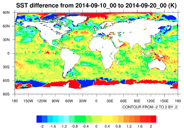
In this plot, we have masked out the SST differences over land, since the values of the field
over land are not representative of actual SST differences, but may represent differences in,
e.g., skin temperature or 2-m air temperature, depending on the source of the SST analyses.
Assuming that an initial condition file and a surface update file have been
created, we're ready to run the MPAS-Atmosphere model itself!
Working from our 240km_uniform directory, we'll begin by creating
a symbolic link to the atmosphere_model executable that we compiled
in /glade/scratch/${USER}/mpas_tutorial/MPAS-Model. We'll also make copies of the namelist.atmosphere
and streams.atmosphere files as well. Recall from when we compiled the model that there are
stream_list.atmosphere.* files that accompany the streams.atmosphere
file; we'll copy these, too.
$ ln -s /glade/scratch/${USER}/mpas_tutorial/MPAS-Model/atmosphere_model .
$ cp /glade/scratch/${USER}/mpas_tutorial/MPAS-Model/namelist.atmosphere .
$ cp /glade/scratch/${USER}/mpas_tutorial/MPAS-Model/streams.atmosphere .
$ cp /glade/scratch/${USER}/mpas_tutorial/MPAS-Model/stream_list.atmosphere.* .
You'll also recall that there were many look-up tables and other data files that are needed by various
physics parameterizations in the model. Before we can run MPAS-Atmosphere, we'll need to create symbolic links
to these files as well in our working directory:
$ ln -s /glade/scratch/${USER}/mpas_tutorial/MPAS-Model/src/core_atmosphere/physics/physics_wrf/files/* .
Before running the model, we will need to edit the namelist.atmosphere file,
which is the namelist for the MPAS-Atmosphere model itself. The default
namelist.atmosphere is set up for a 120-km mesh; in order to run the model
on a different mesh, there is one key parameter that depends on the model resolution:
- config_dt — the model integration time step (delta-t), in seconds.
As will be described in the lectures, the model integration step is generally chosen based on
the finest horizontal resolution in a simulation domain.
To tell the model the date and time at which integration will begin (important, e.g., for computing
solar radiation parameters), and to specify the length of the integration to be run, there are
two other parameters that must be set for each simulation:
- config_start_time — the start time of the integration.
- config_run_duration — the length of the integration.
Lastly, when running the MPAS-Atmosphere model in parallel, we must tell the model the prefix
of the filenames that contain mesh partitioning information for different MPI task counts:
- config_block_decomp_file_prefix — the file prefix (to be suffixed with processor count)
of the file containing mesh partitioning information.
Accordingly, we must edit at least these parameters in the namelist.atmosphere file; other
parameters are described in Appendix B of the MPAS-Atmosphere Users' Guide, and do not necessarily
need to be changed:
&nhyd_model
    config_dt = 1200.0
    config_start_time = '2014-09-10_00:00:00'
    config_run_duration = '5_00:00:00'
/

&decomposition
    config_block_decomp_file_prefix = 'x1.10242.graph.info.part.'
/
For a relatively coarse mesh like the 240-km mesh, we can also call the radiation schemes less frequently
to allow the model to run a little more quickly. Let's set the radiation calling interval to 1 hour:
&physics
    config_radtlw_interval = '01:00:00'
    config_radtsw_interval = '01:00:00'
/
After changing the parameters shown above in the namelist.atmosphere file, we must also set
the name of the initial condition file, the name of the surface update file, and the interval
at which we would like to read the surface update file in the streams.atmosphere file:
<immutable_stream name="input"
                  type="input"
                  filename_template="x1.10242.init.nc"
                  input_interval="initial_only"/>

<stream name="surface"
        type="input"
        filename_template="x1.10242.sfc_update.nc"
        filename_interval="none"
        input_interval="86400">

    <file name="stream_list.atmosphere.surface"/>

</stream>
Having set up the namelist.atmosphere and streams.atmosphere files,
we're almost ready to run the model in parallel. You'll recall from the lectures that we need to supply
a graph partition file to tell MPAS how the horizontal domain is partitioned among MPI tasks. Accordingly,
we'll create a symbolic link to the partition file for
36 MPI tasks for the 240-km mesh in our working directory:
$ ln -s /glade/p/mmm/wmr/mpas_tutorial/meshes/x1.10242.graph.info.part.36 .
As a general rule, a mesh with N
grid columns should be run on at most N/160 processors in MPAS-Atmosphere to make
efficient use of the processors. So, for the mesh in this exercise, which has 10242 grid
columns, we could in principle use up to about 64 MPI tasks while still making relatively
efficient use of the computing resources. For this exercise, however, we will use a single,
full Cheyenne node with 36 cores.
Now, we should be able to run MPAS using 36 MPI tasks. Before submitting a job with qsub,
we can copy a prepared job script to our working directory.
$ cp /glade/p/mmm/wmr/mpas_tutorial/job_scripts/run_model.pbs .
$ qsub run_model.pbs
We can check on the status of our job with qstat -u $USER. Once the model
begins to run, it will write information about its progress to
the log.atmosphere.0000.out file. We can use tail -f
to follow the updates to the log file as the model runs:
$ tail -f log.atmosphere.0000.out
If the model has started up successfully and begun to run, we should see messages
like this
 Begin timestep 2014-09-10_06:00:00
 --- time to run the LW radiation scheme L_RADLW =T
 --- time to run the SW radiation scheme L_RADSW =T
 --- time to run the convection scheme L_CONV    =T
 --- time to apply limit to accumulated rainc and rainnc L_ACRAIN   =F
 --- time to apply limit to accumulated radiation diags. L_ACRADT   =F
 --- time to calculate additional physics_diagnostics               =F
  split dynamics-transport integration 3

 global min, max w -0.177687 0.512867
 global min, max u -112.127 112.008
  Timing for integration step: 5.78077 s
written for each timestep that the model takes. If not, a log.atmosphere.0000.err
file may have been created, and if so, it may have messages to indicate what might have gone wrong.
The model simulation should take less than about a five minutes to complete.
As the model runs, you may notice
that several netCDF output files are being created:
- diag.2014.09.*.nc — These files contain mostly 2-d diagnostic fields that were listed in the stream_list.atmosphere.diagnostics file.
- history.2014.09.*.nc — These files contain mostly 3-d prognostic and diagnostic fields from the model.
- restart.2014.09.*.nc — These are model restart files that are essentially checkpoints of the model state; a simulation can be re-started from any of these checkpoint/restart files.
If the model has successfully begun running, we can move to the next sub-section to obtain and compile
the convert_mpas utility for interpolating model output files to a lat-lon
grid for quick visualization.
We saw in earlier sections that Python scripts may be used to visualize fields in MPAS
netCDF files. Although these scripts can produce publication-quality figures, many
times all that is needed is a way to quickly inspect the fields in a file.
The convert_mpas program is designed to interpolate
fields from the unstructured MPAS mesh to a regular lat-lon grid for easy checking,
e.g., with ncview.
As with the MPAS-Model code, the convert_mpas code may be
obtained most easily by cloning a GitHub repository. Working from our /glade/scratch/${USER}/mpas_tutorial directory,
we'll download the code in this way:
$ cd /glade/scratch/${USER}/mpas_tutorial
$ git clone https://github.com/mgduda/convert_mpas.git
$ cd convert_mpas
The convert_mpas utility is compiled via a simple Makefile.
In general, one can edit the Makefile in the main convert_mpas
directory.
We can build the convert_mpas utility by simply running make
with no command-line arguments:
$ make
If compilation was successful, there should now be an executable file named convert_mpas.
So that we can run this program from any of our working directories, we'll add our current directory to our
shell ${PATH} environment variable:
$ export PATH=/glade/scratch/${USER}/mpas_tutorial/convert_mpas:${PATH}
You may like to take a few minutes to read through the README.md file to familiarize
yourself with the usage of the convert_mpas program. We'll have a chance to exercise
the convert_mpas utility in the next section.
In the previous section, we were able to make a five-day, real-data simulation on
a 240-km quasi-uniform mesh. In this section, we'll practice preparing a variable-resolution,
240km – 48km mesh with the grid_rotate tool, after which we'll
proceed as we did for the quasi-uniform case to process static, terrestrial fields on this
variable-resolution mesh.
As we saw in the first section, processing the static fields can take some time, so while
this processing is taking place, we'll practice using the convert_mpas
tool to interpolate output from our 240-km quasi-uniform simulation to a lat-lon grid for
quick visualization.
Once the static field processing has completed for the 240km – 48km variable-resolution mesh,
we'll interpolate the initial conditions fields and start a simulation on this mesh. This
simulation will take about half an hour to complete, so we'll want to get this running so that it
will have completed by the next section.
A common theme with MPAS is the need to obtain source code from git
repositories hosted on GitHub. The grid_rotate utility
is no exception in this regard. One difference, however, is that the grid_rotate
code is contained in a repository that houses many different tools for MPAS cores,
including the MPAS-Albany Land Ice core, the MPAS-Ocean core, and the MPAS-Sea Ice core.
The grid_rotate utility is found in the MPAS-Tools repository,
which we can clone into our mpas_tutorial working directory
with the following commands:
$ cd /glade/scratch/${USER}/mpas_tutorial
$ git clone https://github.com/MPAS-Dev/MPAS-Tools.git
Within the MPAS-Tools repository, the grid_rotate code resides
in the mesh_tools/grid_rotate sub-directory. We can change to
this directory and build the grid_rotate
utility with the make command.
$ cd MPAS-Tools/mesh_tools/grid_rotate
$ make
So that we can more easily run the grid_rotate program from any working directory, we'll add
our current working directory to our shell ${PATH}.
$ export PATH=/glade/scratch/${USER}/mpas_tutorial/MPAS-Tools/mesh_tools/grid_rotate:${PATH}
Now that we have a means of rotating the location of refinement in a variable-resolution MPAS
mesh, we can begin the process of preparing such a mesh. For this tutorial, we'll be using
a mesh that refines from 240-km grid spacing down to about 48-km grid spacing over an elliptic
region.
When creating initial conditions and running the 240-km quasi-uniform simulation, we worked
in a sub-directory named 240km_uniform. For our variable-resolution
simulation, we'll work in a sub-directory named 240-48km_variable
to keep our work separated. Let's create the 240-48km_variable directory
and link in the variable-resolution mesh from /glade/p/mmm/wmr/mpas_tutorial/meshes into that directory:
$ cd /glade/scratch/${USER}/mpas_tutorial
$ mkdir 240-48km_variable
$ cd 240-48km_variable
$ ln -s /glade/p/mmm/wmr/mpas_tutorial/meshes/x5.30210.grid.nc .
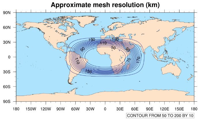
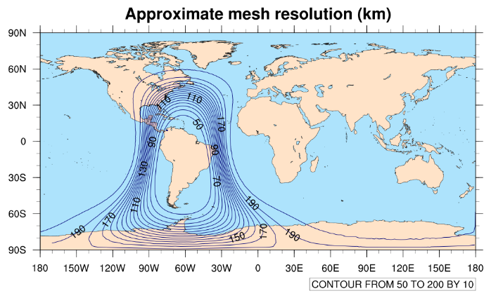
The x5.30210.grid.nc mesh contains 30210 grid cells and refines by
a factor of five (from 240-km grid spacing to 48-km grid spacing). The refinened region is
centered over (0.0 lat, 0.0 lon), and we can get a quick idea of the size of the refinement
by plotting contours of the approximate mesh resolution with
the mesh_resolution.ncl NCL script:
$ cp /glade/p/mmm/wmr/mpas_tutorial/ncl_scripts/mesh_resolution.ncl .
$ export FNAME=x5.30210.grid.nc
$ ncl mesh_resolution.ncl
When running the mesh_resolution.ncl script, a plot like
the one below should be produced in a file named 'mesh_resolution.png', and which
you can view with the display command:
$ display mesh_resolution.png
Using the grid_rotate tool, we can change the location and orientation
of this refinement to an area of our choosing. Before running the grid_rotate
program, we need a copy of the input namelist that is read by this program:
$ cp /glade/scratch/${USER}/mpas_tutorial/MPAS-Tools/mesh_tools/grid_rotate/namelist.input .
As described in the lectures, we'll set the parameters in the namelist.input
file to relocate the refined region in the mesh. For example, to move the refinement over South America,
we might use:
&input
   config_original_latitude_degrees = 0
   config_original_longitude_degrees = 0

   config_new_latitude_degrees = -19.5
   config_new_longitude_degrees = -62
   config_birdseye_rotation_counter_clockwise_degrees = 90
/
Feel free to place the refinement wherever you would like!
After making changes to the namelist.input file, we can rotate
the x5.30210.grid.nc file to create a new "grid" file with any name
we choose. For example:
$ grid_rotate x5.30210.grid.nc SouthAmerica.grid.nc
As with the original x5.30210.grid.nc file, we can plot the approximate
resolution of our rotated grid file with commands like the following:
$ export FNAME=SouthAmerica.grid.nc
$ ncl mesh_resolution.ncl
Of course, the name SouthAmerica.grid.nc should be replaced with the name that
you have chosen for your rotated grid when setting the FNAME environment
variable. In our example, the resulting plot looks like the one below.
It may take some iteration to get the refinement just where you would like it. You can go back and
edit namelist.input file, then re-run the grid_rotate
program, and finally, re-run the ncl mesh_resolution.ncl command until
you are satisfied!
Interpolating static, geographical fields to a variable-resolution MPAS mesh works
in essentially the same way as it does for a quasi-uniform mesh. So, the steps taken
in this section should seem familiar — they mirror what we did in Section 1.3!
To begin the process, we'll symbolically link the init_atmosphere_model
executable into our 240-48km_variable directory, and we'll copy
the default namelist.init_atmosphere and streams.init_atmosphere
files as well:
$ ln -s /glade/scratch/${USER}/mpas_tutorial/MPAS-Model/init_atmosphere_model .
$ cp /glade/scratch/${USER}/mpas_tutorial/MPAS-Model/namelist.init_atmosphere .
$ cp /glade/scratch/${USER}/mpas_tutorial/MPAS-Model/streams.init_atmosphere .
As before, we'll set the following variables in the namelist.init_atmosphere file:
&nhyd_model
    config_init_case = 7
/
&data_sources
    config_geog_data_path = '/glade/p/mmm/wmr/mpas_tutorial/mpas_static/'
    config_landuse_data = 'MODIFIED_IGBP_MODIS_NOAH'
    config_topo_data = 'GMTED2010'
    config_vegfrac_data = 'MODIS'
    config_albedo_data = 'MODIS'
    config_maxsnowalbedo_data = 'MODIS'
    config_supersample_factor = 3
/
&preproc_stages
    config_static_interp = true
    config_native_gwd_static = true
    config_vertical_grid = false
    config_met_interp = false
    config_input_sst = false
    config_frac_seaice = false
/
In editing the streams.init_atmosphere file, we'll choose
the filename for the "input" stream to match whatever name we chose for our rotated
grid file:
<immutable_stream name="input"
                  type="input"
                  filename_template="SouthAmerica.grid.nc"
                  input_interval="initial_only"/>
and we'll set the filename for the "output" stream to follow the same
naming convention, but using "static" instead of "grid":
<immutable_stream name="output"
                  type="output"
                  filename_template="SouthAmerica.static.nc"
                  packages="initial_conds"
                  output_interval="initial_only" />
With these changes, we're ready to run the init_atmosphere_model program.
In order to submit the job to the queuing system, we can copy the same prepared job script as in
Section 1.3 and submit it with qsub:
$ cp /glade/p/mmm/wmr/mpas_tutorial/job_scripts/init_real.pbs .
$ qsub init_real.pbs
As before, processing of the static, geographical fields may take roughly 30 – 45 minutes to complete.
While the static, geographical fields are being processed for our 240km – 48km variable-resolution
mesh, we can experiment with the use of the convert_mpas utility to interpolate
output from our 240-km, quasi-uniform simulation.
If you didn't have a chance to download and compile the convert_mpas program
back in Section 2.4, you will need to go back to that section before proceeding with the rest of this
section.
We'll change directories to the 240km_uniform directory, and we
may also need to add the directory containing the convert_mpas utility to our
shell ${PATH} variable again:
$ cd /glade/scratch/${USER}/mpas_tutorial/240km_uniform
$ export PATH=/glade/scratch/${USER}/mpas_tutorial/convert_mpas:${PATH}
In the 240km_uniform directory, we should see output files from MPAS that
are named history*nc and diag*nc:
$ ls -l history*nc diag*nc
-rw-r--r-- 1 duda ncar  4525528 Apr  8 23:56 diag.2014-09-10_00.00.00.nc
-rw-r--r-- 1 duda ncar  4525528 Apr  8 23:56 diag.2014-09-10_03.00.00.nc
...
-rw-r--r-- 1 duda ncar  4525528 Apr  8 23:59 diag.2014-09-14_21.00.00.nc
-rw-r--r-- 1 duda ncar  4525528 Apr  8 23:59 diag.2014-09-15_00.00.00.nc
-rw-r--r-- 1 duda ncar 94449804 Apr  8 23:56 history.2014-09-10_00.00.00.nc
-rw-r--r-- 1 duda ncar 94449804 Apr  8 23:56 history.2014-09-10_06.00.00.nc
...
-rw-r--r-- 1 duda ncar 94449804 Apr  8 23:59 history.2014-09-14_18.00.00.nc
-rw-r--r-- 1 duda ncar 94449804 Apr  8 23:59 history.2014-09-15_00.00.00.nc
As a first try, we can interpolate the fields from the final model "history" file,
history.2014-09-15_00.00.00.nc, to a 0.5-degree lat-lon grid
with the command:
$ convert_mpas history.2014-09-15_00.00.00.nc
The interpolation should take less than a minute, and the result should be a file named latlon.nc.
Let's take a look at this file with the ncview utility:
$ ncview latlon.nc
After launching ncview we can, e.g., view the qv field, which may look something
like the plot below at the lowest model level.
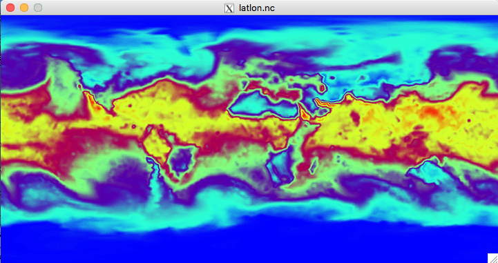
Feel free to browse some of the other fields in the file by selecting them from the "2d vars" and "3d vars" buttons.
All of the fields are described in Appendix D of the User's Guide.
When we're done viewing the latlon.nc file, we'll delete it. The convert_mpas
utility attempts to append to existing latlon.nc files when converting a new MPAS netCDF file,
and this often doesn't work as expected, so to avoid confusion, it's best to remove the
latlon.nc file we just created with
$ rm latlon.nc
before converting another MPAS output file.
As we just saw, it can take upwards of a minute to interpolate a single MPAS "history" file. If we are only interested
in a small subset of the fields in an MPAS file, we can restrict the interpolation to just those fields by providing
a file named include_fields in our working directory.
Using an editor of your choice, create a new text file named include_fields with the following
contents:
u10
v10
precipw
After saving the file, we can re-run the convert_mpas program as before to produce
a latlon.nc file with just the 10-meter surface winds and precipitable water:
$ convert_mpas history.2014-09-15_00.00.00.nc
$ ncview latlon.nc
The convert_mpas program should have taken just a few seconds to run; if not, make
sure the latlon.nc file was deleted before re-running convert_mpas.
The only fields in the new latlon.nc file should be "precipw", "u10", and "v10".
Rather than converting just a single file at a time, we can convert multiple MPAS output files and write the results
to the same latlon.nc file. The key to doing this is to use the first command-line argument
to convert_mpas to specify a file that contains horizontal (SCVT) mesh information, and to
let subsequent command-line arguments specify MPAS netCDF files that contain fields to be remapped.
To interpolate the "precipw", "u10", and "v10" fields for our entire 5-day simulation, we can use the following
commands:
$ rm latlon.nc
$ convert_mpas x1.10242.init.nc history.*.nc
$ ncview latlon.nc
Note, again, that the first command-line argument to convert_mpas is only used to obtain
SCVT mesh information by the convert_mpas program when multiple command-line arguments
are given, and all remaining command-line arguments specify netCDF files with fields to be interpolated!
When viewing a netCDF file with multiple time records, you can step through the time periods in
ncview with the "forward" and "backward" buttons to the right and left
of the "pause" button:

As a final exercise in viewing MPAS output via the convert_mpas and ncview
programs, we'll zoom in on a part of the globe, looking at the 250 hPa vertical vorticity field over East Asia on a 1/10-degree
lat-lon grid.
To do this, we will first need to edit the include_fields file so that it contains
just the following line:
vorticity_250hPa
Then, we'll create a new file named target_domain with the editor of our choice. This file
should contain the following lines:
startlat=30
endlat=60
startlon=90
endlon=150
nlat=300
nlon=600
After editing the include_fields file and creating the target_domain
file, we can remove the old latlon.nc file and use the convert_mpas
program to interpolate the 250 hPa vorticity field from our diag.*.nc files:
$ rm latlon.nc
$ convert_mpas x1.10242.init.nc diag*nc
$ ncview latlon.nc
If the processing of the static, geographical fields for the 240km – 48km variable-resolution mesh has not
finished, yet, you can feel free to experiment more with the convert_mpas program!
Once the processing of the static, geographical fields has completed in the 240-48km_variable
directory, we should have a new "static" file as well as a log.init_atmosphere.0000.out
file. In our example, the static file is named SouthAmerica.static.nc, but your
file should have whatever name was specified in the definition of the "output" stream in
the streams.init_atmosphere file.
Before proceeding, it's a good idea to verify that there were no errors reported in
the log.init_atmosphere.0000.out file. We can also make a plot of the terrain height
field as we did for the 240-km quasi-uniform simulation:
$ cp /glade/p/mmm/wmr/mpas_tutorial/python_scripts/plot_terrain.py .
$ ./plot_terrain.py SouthAmerica.static.nc
Once we have convinced ourselves that the static, geographical processing was successful, we can proceed as
we did for the 240-km quasi-uniform simulation. We'll create a symbolic link to the ERA5
intermediate file valid at 0000 UTC on 10 September 2014:
$ ln -s /glade/p/mmm/wmr/mpas_tutorial/met_data/ERA5:2014-09-10_00 .
As before, we'll set up the namelist.init_atmosphere file to instruct
the init_atmosphere_model program to interpolate meteorological and land-surface
initial conditions:
&nhyd_model
    config_init_case = 7
    config_start_time = '2014-09-10_00:00:00'
/
&dimensions
    config_nvertlevels = 41
    config_nsoillevels = 4
    config_nfglevels = 38
    config_nfgsoillevels = 4
/
&data_sources
    config_met_prefix = 'ERA5'
    config_use_spechumd = false
/
&vertical_grid
    config_ztop = 30000.0
    config_nsmterrain = 1
    config_smooth_surfaces = true
    config_dzmin = 0.3
    config_nsm = 30
    config_tc_vertical_grid = true
    config_blend_bdy_terrain = false
/
&interpolation_control
    config_extrap_airtemp = 'lapse-rate'
/
&preproc_stages
    config_static_interp = false
    config_native_gwd_static = false
    config_vertical_grid = true
    config_met_interp = true
    config_input_sst = false
    config_frac_seaice = true
/
Besides the namelist.init_atmosphere file, we must also edit the XML
I/O configuration file, streams.init_atmosphere, to specify the name
of the static file that will serve as input to the init_atmosphere_model program, as well as
the name of the MPAS-Atmosphere initial condition file to be created. Specifically, we must set
the filename_template for the "input" stream to the name of our static file:
<immutable_stream name="input"
                  type="input"
                  filename_template="SouthAmerica.static.nc"
                  input_interval="initial_only"/>
and we must set the name of the initial condition file to be created in the "output" stream:
<immutable_stream name="output"
                  type="output"
                  filename_template="SouthAmerica.init.nc"
                  packages="initial_conds"
                  output_interval="initial_only" />
After editing the namelist.init_atmosphere and streams.atmosphere
files, and linking the intermediate file to our run directory, we can run
the init_atmosphere_model
program with qcmd:
$ qcmd -A UMMM0004 -- ./init_atmosphere_model
The init_atmosphere_model program should take just a few minutes to run.
Once the init_atmosphere_model program finishes, as always, it is best to verify that there were
no error messages reported in the log.init_atmosphere.0000.out file. We should also have a file
whose name matches the filename we specified for the "output" stream in the streams.init_atmosphere
file. In our example, we should have a file named SouthAmerica.init.nc.
If all was successful, we are ready to run a variable-resolution MPAS simulation. For this simulation, we won't prepare
an SST and sea-ice surface update file for the model; however, if you would like to try doing so following what was done
in Section 2.2, feel free to do so!
Assuming that an initial condition file, and, optionally, a surface update file have been
created, we're ready to run a variable-resolution, 240km – 48km simulation with refinement
over a part of the globe that interests us.
As a first step, you may recall that we need to create symbolic links to the atmosphere_model
executable, as well as to the physics look-up tables, into our working directory:
$ ln -s /glade/scratch/${USER}/mpas_tutorial/MPAS-Model/atmosphere_model .
$ ln -s /glade/scratch/${USER}/mpas_tutorial/MPAS-Model/src/core_atmosphere/physics/physics_wrf/files/* .
We will also need copies of the namelist.atmosphere,
streams.atmosphere, and stream_list.atmosphere.*
files:
$ cp /glade/scratch/${USER}/mpas_tutorial/MPAS-Model/namelist.atmosphere .
$ cp /glade/scratch/${USER}/mpas_tutorial/MPAS-Model/streams.atmosphere .
$ cp /glade/scratch/${USER}/mpas_tutorial/MPAS-Model/stream_list.atmosphere.* .
Next, we will need to edit the namelist.atmosphere file. Recall from
before that the default namelist.atmosphere is set up for a 120-km mesh;
in order to run the model on a different mesh, there is one key key parameter that depends on
the model resolution:
- config_dt — the model integration time step (delta-t), in seconds.
The model timestep, config_dt must be set to a value that is appropriate
for the smallest grid distance in the mesh. In our case, we need to choose a time step that is
suitable for a 48-km grid distance; a value of 240 seconds is reasonable. In the lecture on MPAS
dynamics we will say more about how to choose the model timestep.
To tell the model the date and time at which integration will begin, and to specify the length
of the integration to be run, there are two other parameters that must be set for each simulation:
- config_start_time — the start time of the integration.
- config_run_duration — the length of the integration.
In order to make maximal use of the time between this practical session and the next, we'll try
to run a 5-day simulation starting on 2014-09-10_00.
Lastly, when running the MPAS-Atmosphere model in parallel, we must tell the model the prefix
of the filenames that contain mesh partitioning information for different MPI task counts:
- config_block_decomp_file_prefix — the file prefix (to be suffixed with processor count)
of the file containing mesh partitioning information.
For the 240km – 48km variable-resolution mesh, we can find a mesh partition file with 36 partitions
at /glade/p/mmm/wmr/mpas_tutorial/meshes/x5.30210.graph.info.part.36. Let's symbolically link that file
to our run directory now before specifying a value of 'x5.30210.graph.info.part.'
for the config_block_decomp_prefix in our namelist.atmosphere file.
$ ln -s /glade/p/mmm/wmr/mpas_tutorial/meshes/x5.30210.graph.info.part.36 .
Before reading further, you may wish to try making the changes to the namelist.atmosphere
yourself. Once you've done so, you can verify that the options highlighted below match the changes you have made.
&nhyd_model
    config_dt = 240.0
    config_start_time = '2014-09-10_00:00:00'
    config_run_duration = '5_00:00:00'
/
&decomposition
    config_block_decomp_file_prefix = 'x5.30210.graph.info.part.'
/
After changing the parameters shown above in the namelist.atmosphere file, we must also set
the name of the initial condition file in the streams.atmosphere file:
<immutable_stream name="input"
                  type="input"
                  filename_template="SouthAmerica.init.nc"
                  input_interval="initial_only"/>
Optionally, if you decided to create an SST update file for this variable-resolution simulation
in the previous section, you can also edit the "surface" stream in the streams.atmosphere
file to specify the name of that surface update file, as well as the interval at which the model
should read updates from it:
<stream name="surface"
        type="input"
        filename_template="SouthAmerica.sfc_update.nc"
        filename_interval="none"
        input_interval="86400">

    <file name="stream_list.atmosphere.surface"/>

</stream>
Having set up the namelist.atmosphere and streams.atmosphere
files, we're ready to run the model in parallel.
We can copy the same job script as we used for the quasi-uniform
240-km simulation and submit it as usual with qsub.
$ cp /glade/p/mmm/wmr/mpas_tutorial/job_scripts/run_model.pbs .
$ qsub run_model.pbs
Once the model begins to run, you may like to "tail" the log.atmosphere.0000.out
file with the "-f" option to follow the progress of the MPAS simulation:
$ tail -f log.atmosphere.0000.out
If the model has started up successfully and begun to run, we should see messages
like this:
 Begin timestep 2014-09-10_00:12:00
 --- time to run the LW radiation scheme L_RADLW =F
 --- time to run the SW radiation scheme L_RADSW =F
 --- time to run the convection scheme L_CONV    =T
 --- time to apply limit to accumulated rainc and rainnc L_ACRAIN   =F
 --- time to apply limit to accumulated radiation diags. L_ACRADT   =F
 --- time to calculate additional physics_diagnostics               =F
  split dynamics-transport integration 3

 global min, max w -1.06611 0.722390
 global min, max u -117.781 118.251
  Timing for integration step: 4.18681 s
This simulation will take about half an hour to run. Now may be a convenient time to ask any questions that you may have!
Having gained experience in running global simulations, we are now well positioned to
run a limited-area (i.e., a regional) simulation with MPAS-Atmosphere. We will begin
by defining the simulation domain using the MPAS-Limited-Area tool to cover any part
of the globe that interests us. Then, we will subset the "static" fields from an existing
60-km quasi-uniform static file.
Once we are satisfied with the geographic coverage of our regional static fields, we
will interpolate initial and lateral boundary conditions from the 0.5-degree CFSv2 datset.
Given ICs and LBCs for our regional domain, we can begin running a 3-day regional
simulation from 2019-09-01 0000 UTC through 2019-09-04 0000 UTC.
After our simulation has run (or, even after the first few model output files are
available), we will practice using NCL and the convert_mpas tool to visualize
the regional output.
To begin the work of defining a regional simulation domain for MPAS-Atmosphere, we will
first obtain a copy of the MPAS-Limited-Area tool. As with the MPAS model code and MPAS-Tools
code, we will clone the MPAS-Limited-Area repository from GitHub. From within our /glade/scratch/${USER}/mpas_tutorial
directory, we can do this with the following commands:
$ cd /glade/scratch/${USER}/mpas_tutorial
$ git clone https://github.com/MPAS-Dev/MPAS-Limited-Area.git
After changing to the MPAS-Limited-Area directory that
should have been created by the git clone command, we
can prepare a file describing our desired regional domain. Depending on the type
of region that we intend to define (circular, elliptical, channel, or polygon),
we can use any of the example region definition files in the docs/points-examples/ sub-directory as a starting point.
For the purpose of illustration, we'll use the japan.ellipse.pts
file from docs/points-examples/ as a starting point to set up
an elliptical domain over the Mediterranean Sea; however, you may set up your
regional domain over any other part of the globe using any of the available region types.
After copying this file to a file named mediterranean.pts in our
current working directory with
$ cp docs/points-examples/japan.ellipse.pts mediterranean.pts
we can edit the file so that its contents look like the following:
Name: Mediterranean
Type: ellipse
Point: 37.9, 18.0
Semi-major-axis: 3200000
Semi-minor-axis: 1700000
Orientation-angle: 100
Again, you can set up any alternative regional domain as you prefer — the Mediterranean
domain is only used here as an example!
To aid in locating your regional domain, it may be helpful to use
OpenStreetMap, where you can right-click
anywhere on a map and choose "Show address" to find the latitude and longitude of a point.
Having prepared a region definition file, we can use the create_region
tool to create a subset of an existing global "static" file for our specified region. We can symbolically
link a global, quasi-uniform, 60-km static file to our working directory with:
$ ln -s /glade/p/mmm/wmr/mpas_tutorial/meshes/x1.163842.static.nc .
Then, we can create a regional static file with a command like:
$ ./create_region mediterranean.pts x1.163842.static.nc
The create_region tool should take just a few seconds to run, and the result
should be a new static file and a new graph.info file, named according to
the "Name" we specified in our region defintion file, e.g,:
Mediterranean.static.nc
Mediterranean.graph.info
At this point, we may like to plot one of the time-invariant, terrestrial fields from our new regional
static file. We can plot the terrain height field using an NCL script, regional_terrain.ncl,
which we will first copy to our working directory:
$ cp /glade/p/mmm/wmr/mpas_tutorial/ncl_scripts/regional_terrain.ncl .
This NCL script uses a custom color map. In order for NCL to find this color map, we'll need to set the NCARG_COLORMAPS
environment variable as follows:
$ export NCARG_COLORMAPS=/glade/p/mmm/wmr/mpas_tutorial/ncl_colormaps/:$NCARG_ROOT/lib/ncarg/colormaps/
Before running the script, we will also need to set the latitude and longitude view point for the orthographic projection used
by the script. In the regional_terrain.ncl script, locate the section that looks like the following,
and modify the cenlat and cenlon values so that they coincide roughly with
the center of your regional domain.
;;;;;;;;;;;;;;;;;;;;;;;;;;;;;;;;;;;;;;;;;;;;;;;;;;;;;;;;;;;;;;;;;;;;;;;;;;;;;;;;
;
; Main script
;
;;;;;;;;;;;;;;;;;;;;;;;;;;;;;;;;;;;;;;;;;;;;;;;;;;;;;;;;;;;;;;;;;;;;;;;;;;;;;;;;
begin

  ;
  ; Center latitude and longitude
  ;
  cenlat = 0.0
  cenlon = 0.0
Additionally, we will need to set the GNAME environment variable to the name of our regional
static file; e.g., for our Mediterranean example:
$ export GNAME=Mediterranean.static.nc
We can then run the script with
$ ncl regional_terrain.ncl
to produce a PNG image that should look something like the following:
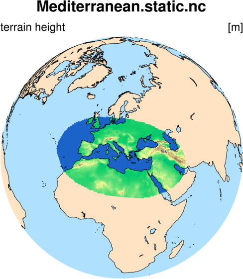
Before proceeding to the next section, you may need to iterate between (1) modifying your region definition file,
(2) running the create_region tool to create a new netCDF file, and (3) plotting the new
regional terrain field with the regional_terrain.ncl script.
Now that we have a regional static file for our domain of interest, we can
prepare initial conditions for this domain in essentially the same way as we
prepared initial conditions for global simulations. The key difference is
that we will blend the terrain field along the regional domain boundaries
with the terrain from our initial conditions data.
Let's create a new directory in /glade/scratch/${USER}/mpas_tutorial to run our regional simulation:
$ mkdir /glade/scratch/${USER}/mpas_tutorial/regional
$ cd /glade/scratch/${USER}/mpas_tutorial/regional
We can then move the regional static file and graph.info
files that we created in Section 4.1 to this directory:
$ mv /glade/scratch/${USER}/mpas_tutorial/MPAS-Limited-Area/Mediterranean.static.nc .
$ mv /glade/scratch/${USER}/mpas_tutorial/MPAS-Limited-Area/Mediterranean.graph.info .
As with the global simulations from earlier sessions, we will need to link the init_atmosphere_model
executable to our run directory, and we will also need to copy the namelist.init_atmosphere
and streams.atmosphere files, which we will modify for our regional domain.
$ ln -s /glade/scratch/${USER}/mpas_tutorial/MPAS-Model/init_atmosphere_model .
$ cp /glade/scratch/${USER}/mpas_tutorial/MPAS-Model/namelist.init_atmosphere .
$ cp /glade/scratch/${USER}/mpas_tutorial/MPAS-Model/streams.init_atmosphere .
For our regional simulation, we will use 0.5-degree CFSv2 data valid on 2019-09-01 0000 UTC for initial conditions.
We can symbolically link the CFSV2 intermediate file to our run directory as follows:
$ ln -s /glade/p/mmm/wmr/mpas_tutorial/met_data/CFSV2:2019-09-01_00 .
Unlike in past exercises, we can also try interpolating the initial conditions using multiple MPI tasks. Recall that we use
the Metis tool to create mesh partition files for a specified number of MPI tasks. Using Metis's gpmetis
tool, we can create a partition file for 36 MPI tasks from the Mediterranean.graph.info file that
was generated by MPAS-Limited-Area. The following command should be work:
$ gpmetis -minconn -contig -niter=200 Mediterranean.graph.info 36
Even if we choose not to interpolate the initial conditions in parallel, we will ultimately need the mesh partition file to run
the model in parallel.
Now, we are ready to edit our namelist.init_atmosphere and streams.init_atmosphere
files. To test your understanding, you may like to first try preparing these files yourself for the creation of initial
conditions for your regional domain. Once you've finished editing these files, you can compare against the changes highlighted
below (click on the light blue header bars). Remember that your static file and graph.info file may
have different names, depending on where your regional domain is located.
&nhyd_model
    config_init_case = 7
    config_start_time = '2019-09-01_00:00:00'
    config_stop_time = '2010-10-23_00:00:00'
    config_theta_adv_order = 3
    config_coef_3rd_order = 0.25
/
&dimensions
    config_nvertlevels = 55
    config_nsoillevels = 4
    config_nfglevels = 38
    config_nfgsoillevels = 4
/
&data_sources
    config_geog_data_path = '/glade/p/mmm/wmr/mpas_tutorial/mpas_static/'
    config_met_prefix = 'CFSV2'
    config_sfc_prefix = 'SST'
    config_fg_interval = 86400
    config_landuse_data = 'MODIFIED_IGBP_MODIS_NOAH'
    config_topo_data = 'GMTED2010'
    config_vegfrac_data = 'MODIS'
    config_albedo_data = 'MODIS'
    config_maxsnowalbedo_data = 'MODIS'
    config_supersample_factor = 3
    config_use_spechumd = false
/
&vertical_grid
    config_ztop = 30000.0
    config_nsmterrain = 1
    config_smooth_surfaces = true
    config_dzmin = 0.3
    config_nsm = 30
    config_tc_vertical_grid = true
    config_blend_bdy_terrain = true
/
&interpolation_control
    config_extrap_airtemp = 'lapse-rate'
/
&preproc_stages
    config_static_interp = false
    config_native_gwd_static = false
    config_vertical_grid = true
    config_met_interp = true
    config_input_sst = false
    config_frac_seaice = true
/
&io
    config_pio_num_iotasks = 0
    config_pio_stride = 1
/
&decomposition
    config_block_decomp_file_prefix = 'Mediterranean.graph.info.part.'
/
<streams>
<immutable_stream name="input"
                  type="input"
                  filename_template="Mediterranean.static.nc"
                  input_interval="initial_only" />

<immutable_stream name="output"
                  type="output"
                  filename_template="Mediterranean.init.nc"
                  packages="initial_conds"
                  output_interval="initial_only" />

<immutable_stream name="surface"
                  type="output"
                  filename_template="x1.40962.sfc_update.nc"
                  filename_interval="none"
                  packages="sfc_update"
                  output_interval="86400" />

<immutable_stream name="lbc"
                  type="output"
                  filename_template="lbc.$Y-$M-$D_$h.$m.$s.nc"
                  filename_interval="output_interval"
                  packages="lbcs"
                  output_interval="3:00:00" />

</streams>
For namelist and streams settings that were not modified, either the default value of the setting is acceptable, or the setting is not used when
interpolating time-varying initial conditions. Now is also a good time to check that you understand why we needed to modify the settings that we
did in the namelist.init_atmosphere and streams.init_atmosphere files.
After checking your modifications to the namelist.init_atmosphere and streams.init_atmosphere
files, above, we can run the init_atmosphere_model program with 36 MPI tasks to create regional initial conditions.
To do this, we can copy a prepared job script to run the init_atmosphere_model program and submit
it with qsub.
$ cp /glade/p/mmm/wmr/mpas_tutorial/job_scripts/init_parallel.pbs .
$ qsub init_parallel.pbs
Once the job completes, as always, it's important to verify that there were no errors during
the execution of the init_atmosphere_model program;
the end of the log.init_atmosphere.0000.out file should report zero errors:
-----------------------------------------
 Total log messages printed:
    Output messages =                  464
    Warning messages =                   6
    Error messages =                     0
    Critical error messages =            0
 -----------------------------------------
If there were no errors, we should now have a regional initial conditions file; for our example regional domain the file should be named
Mediterranean.init.nc. We're now ready to generate lateral boundary conditions for our domain in the next section!
The interpolation of lateral boundary conditions for a regional simulation domain
is conceptually similar to the interpolation of initial conditions: the key differences
are: (1) fields are interpolated at several time periods, and (2) the set of fields
to be interpolated are a subset of those required for initial conditions (they include:
theta, rho, u, w, and moisture species).
We will use the CFSv2 reanalyses for lateral boundary conditions. Three days' worth of
six-hourly CFSv2 fields are available in the /glade/p/mmm/wmr/mpas_tutorial/met_data
directory, and we can symbolically link all of these CFSv2 files to our run directory
with the following command:
$ ln -sf /glade/p/mmm/wmr/mpas_tutorial/met_data/CFSV2* .
All that is needed now is to once again edit the namelist.init_atmosphere
and streams.init_atmosphere files to set up the interpolation of LBCs
using "init case" 9. The relevant settings are highlighted in the sections, below (click the light
blue headers to expand each edited file).
&nhyd_model
    config_init_case = 9
    config_start_time = '2019-09-01_00:00:00'
    config_stop_time = '2019-09-04_00:00:00'
    config_theta_adv_order = 3
    config_coef_3rd_order = 0.25
/
&dimensions
    config_nvertlevels = 55
    config_nsoillevels = 4
    config_nfglevels = 38
    config_nfgsoillevels = 4
/
&data_sources
    config_geog_data_path = '/glade/p/mmm/wmr/mpas_tutorial/mpas_static/'
    config_met_prefix = 'CFSV2'
    config_sfc_prefix = 'SST'
    config_fg_interval = 21600
    config_landuse_data = 'MODIFIED_IGBP_MODIS_NOAH'
    config_topo_data = 'GMTED2010'
    config_vegfrac_data = 'MODIS'
    config_albedo_data = 'MODIS'
    config_maxsnowalbedo_data = 'MODIS'
    config_supersample_factor = 3
    config_use_spechumd = false
/
&vertical_grid
    config_ztop = 30000.0
    config_nsmterrain = 1
    config_smooth_surfaces = true
    config_dzmin = 0.3
    config_nsm = 30
    config_tc_vertical_grid = true
    config_blend_bdy_terrain = false
/
&interpolation_control
    config_extrap_airtemp = 'lapse-rate'
/
&preproc_stages
    config_static_interp = false
    config_native_gwd_static = false
    config_vertical_grid = true
    config_met_interp = true
    config_input_sst = false
    config_frac_seaice = true
/
&io
    config_pio_num_iotasks = 0
    config_pio_stride = 1
/
&decomposition
    config_block_decomp_file_prefix = 'Mediterranean.graph.info.part.'
/
<streams>
<immutable_stream name="input"
                  type="input"
                  filename_template="Mediterranean.init.nc"
                  input_interval="initial_only" />

<immutable_stream name="output"
                  type="output"
                  filename_template="foo.nc"
                  packages="initial_conds"
                  output_interval="initial_only" />

<immutable_stream name="surface"
                  type="output"
                  filename_template="x1.40962.sfc_update.nc"
                  filename_interval="none"
                  packages="sfc_update"
                  output_interval="86400" />

<immutable_stream name="lbc"
                  type="output"
                  filename_template="lbc.$Y-$M-$D_$h.$m.$s.nc"
                  filename_interval="output_interval"
                  packages="lbcs"
                  output_interval="6:00:00" />

</streams>
There are a few points worth making about the changes in the streams.init_atmosphere file.
- Because the interpolation of LBCs is not only a horizontal interpolation to the regional mesh, but also a vertical
interpolation to the vertical coordinate surfaces, the "input" stream must read from a file that contains a valid "zgrid"
field. The initial conditions file contains horizontal and vertical mesh information, and so we use it as the file from
which the "input" stream reads.
- The MPAS stream manager infrastructure will complain if an input stream and an output stream share the same
filename_template, so the filename_template for the "output" stream
must be set to some other filename; since "init case" 9 only writes the "lbc" stream, we can make up any filename we like
for the "output" stream.
- The output_interval for the "lbc" stream must match the value of the
config_fg_interval namelist option. In this regional example, using "21600" or "6:00:00" are
equivalent (we could even specify "360:00" if we would like!).
After having edited our namelist.init_atmosphere and streams.init_atmosphere files,
we are ready to run the init_atmosphere_model program again using 36 MPI tasks.
We can submit the init_parallel.pbs script again with qsub:
$ qsub init_parallel.pbs
After the init_atmosphere_model program completes, it is a good idea (as always!) to verify that
there were no errors reported at the end of the log.init_atmosphere.0000.out file:
 -----------------------------------------
 Total log messages printed:
    Output messages =                 2742
    Warning messages =                   0
    Error messages =                     0
    Critical error messages =            0
 -----------------------------------------
If there were no errors, we should now have "lbc" files in our run directory:
$ ls -l lbc*nc
-rw-r--r-- 1 class112 cbet 15469296 Sep  5 16:37 lbc.2019-09-01_00.00.00.nc
-rw-r--r-- 1 class112 cbet 15469296 Sep  5 16:37 lbc.2019-09-01_06.00.00.nc
-rw-r--r-- 1 class112 cbet 15469296 Sep  5 16:37 lbc.2019-09-01_12.00.00.nc
-rw-r--r-- 1 class112 cbet 15469296 Sep  5 16:37 lbc.2019-09-01_18.00.00.nc
-rw-r--r-- 1 class112 cbet 15469296 Sep  5 16:37 lbc.2019-09-02_00.00.00.nc
-rw-r--r-- 1 class112 cbet 15469296 Sep  5 16:37 lbc.2019-09-02_06.00.00.nc
-rw-r--r-- 1 class112 cbet 15469296 Sep  5 16:37 lbc.2019-09-02_12.00.00.nc
-rw-r--r-- 1 class112 cbet 15469296 Sep  5 16:37 lbc.2019-09-02_18.00.00.nc
-rw-r--r-- 1 class112 cbet 15469296 Sep  5 16:37 lbc.2019-09-03_00.00.00.nc
-rw-r--r-- 1 class112 cbet 15469296 Sep  5 16:37 lbc.2019-09-03_06.00.00.nc
-rw-r--r-- 1 class112 cbet 15469296 Sep  5 16:37 lbc.2019-09-03_12.00.00.nc
-rw-r--r-- 1 class112 cbet 15469296 Sep  5 16:37 lbc.2019-09-03_18.00.00.nc
-rw-r--r-- 1 class112 cbet 15469296 Sep  5 16:37 lbc.2019-09-04_00.00.00.nc
We're now ready to run a regional simulation in the next section!
Given regional initial conditions and lateral boundary conditions, we are almost ready
to run a regional simulation. The only differences from running a global simulation are:
(1) we need to set a namelist option to enable the application of LBCs in each model timestep,
and (2) we need to set up an LBC input stream for the model.
As in previous exercises, we will need to symbolically link the atmosphere_model
executable, as well as the look-up tables used by physics schemes, into our run directory. We can do this
with the following commands:
$ ln -s /glade/scratch/${USER}/mpas_tutorial/MPAS-Model/atmosphere_model .
$ ln -s /glade/scratch/${USER}/mpas_tutorial/MPAS-Model/src/core_atmosphere/physics/physics_wrf/files/* .
We also need copies of the default namelist.atmosphere, streams.atmosphere, and
stream_list.atmosphere.* files, which we will edit for our simulation.
$ cp /glade/scratch/${USER}/mpas_tutorial/MPAS-Model/namelist.atmosphere .
$ cp /glade/scratch/${USER}/mpas_tutorial/MPAS-Model/streams.atmosphere .
$ cp /glade/scratch/${USER}/mpas_tutorial/MPAS-Model/stream_list.atmosphere.* .
As with global simulations, the key namelist parameters that must be modified are:
- config_dt - the model integration timestep; roughly six times the minimum grid distance in km is a reasonable first guess
- config_start_time - the starting time for the simulation
- config_run_duration - the duration of the simulation
- config_block_decomp_file_prefix - the prefix (excluding the final number) of the file providing mesh partition information
Different from global simulations, we must also set the namelist option config_apply_lbcs = true!
You may like to try editing the namelist.atmosphere file yourself before checking
your changes against those highlighted, below (click on the light blue header).
&nhyd_model
    config_time_integration_order = 2
    config_dt = 360.0
    config_start_time = '2019-09-01_00:00:00'
    config_run_duration = '3_00:00:00'
    config_split_dynamics_transport = true
    config_number_of_sub_steps = 2
    config_dynamics_split_steps = 3
    config_horiz_mixing = '2d_smagorinsky'
    config_visc4_2dsmag = 0.05
    config_scalar_advection = true
    config_monotonic = true
    config_coef_3rd_order = 0.25
    config_epssm = 0.1
    config_smdiv = 0.1
/
&damping
    config_zd = 22000.0
    config_xnutr = 0.2
/
&limited_area
    config_apply_lbcs = true
/
&io
    config_pio_num_iotasks = 0
    config_pio_stride = 1
/
&decomposition
    config_block_decomp_file_prefix = 'Mediterranean.graph.info.part.'
/
&restart
    config_do_restart = false
/
&printout
    config_print_global_minmax_vel = true
    config_print_detailed_minmax_vel = false
/
&IAU
    config_IAU_option = 'off'
    config_IAU_window_length_s = 21600.
/
&physics
    config_sst_update = false
    config_sstdiurn_update = false
    config_deepsoiltemp_update = false
    config_radtlw_interval = '00:30:00'
    config_radtsw_interval = '00:30:00'
    config_bucket_update = 'none'
    config_physics_suite = 'mesoscale_reference'
/
&soundings
    config_sounding_interval = 'none'
/
In the streams.atmosphere file, we will need to set the filename_template for the "input" stream to the name of our regional initial conditions file. We will also need to set the input_interval for the "lbc_in" stream to the interval at which we have prepared lateral boundary conditions files.
After editing the streams.atmosphere file, you can compare your changes against
those highlighted, below (click on the light blue header).
<streams>
<immutable_stream name="input"
                  type="input"
                  filename_template="Mediterranean.init.nc"
                  input_interval="initial_only" />

<immutable_stream name="restart"
                  type="input;output"
                  filename_template="restart.$Y-$M-$D_$h.$m.$s.nc"
                  input_interval="initial_only"
                  output_interval="1_00:00:00" />

<stream name="output"
        type="output"
        filename_template="history.$Y-$M-$D_$h.$m.$s.nc"
        output_interval="6:00:00" >

	<file name="stream_list.atmosphere.output"/>
</stream>

<stream name="diagnostics"
        type="output"
        filename_template="diag.$Y-$M-$D_$h.$m.$s.nc"
        output_interval="3:00:00" >

	<file name="stream_list.atmosphere.diagnostics"/>
</stream>

<stream name="surface"
        type="input"
        filename_template="x1.40962.sfc_update.nc"
        filename_interval="none"
        input_interval="none" >

	<file name="stream_list.atmosphere.surface"/>
</stream>

<immutable_stream name="iau"
                  type="input"
                  filename_template="x1.40962.AmB.$Y-$M-$D_$h.$m.$s.nc"
                  filename_interval="none"
                  packages="iau"
                  input_interval="initial_only" />

<immutable_stream name="lbc_in"
                  type="input"
                  filename_template="lbc.$Y-$M-$D_$h.$m.$s.nc"
                  filename_interval="input_interval"
                  packages="limited_area"
                  input_interval="6:00:00" />

</streams>
Once we have finished editing the namelist.atmosphere
and streams.atmosphere files, we're ready to run a simulation.
We can copy the same job script as we used for the quasi-uniform 240-km simulation
and submit it as usual with qsub.
$ cp /glade/p/mmm/wmr/mpas_tutorial/job_scripts/run_model.pbs .
$ qsub run_model.pbs
This simulation will take a while to run.
Once the first few netCDF output files have been produced, even before the full simulation has completed,
we can proceed to the next section to practice visualizing the initial regional model output.
If the regional simulation ran successfully — or even if it has just begun running and has produced
several time periods of output — we can visualize the output using two different methods.
In order to take a quick first look at the output, we can use the convert_mpas
tool to interpolate our output to a regular latitude-longitude grid, after which we can view the interpolated
fields using ncview.
Let's first check whether the path to the convert_mpas program is in our $PATH environment variable with:
$ which convert_mpas
If the "which" command prints something like
/usr/bin/which: no convert_mpas ...
we can set our $PATH environment variable by typing:
$ export PATH=/glade/scratch/${USER}/mpas_tutorial/convert_mpas:$PATH
To start, we can simply interpolate the full set of fields from all diagnostics output files
to a global 0.5-degree lat-lon grid with the following command:
$ convert_mpas Mediterranean.static.nc diag*nc
We can then view the resulting latlon.nc file with ncview:
$ ncview latlon.nc
Because the default target grid for the convert_mpas program is a global,
0.5-degree grid, viewing, e.g., the "precipw" field might look like the image below.
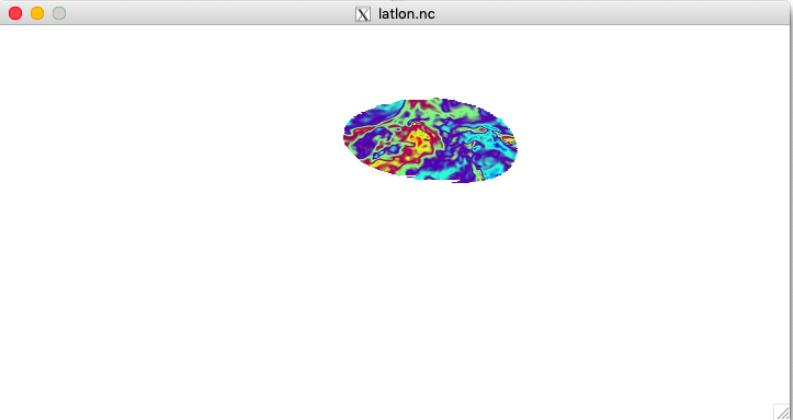
As we did in Section 3.3, we can try to interpolate to a lat-lon grid that is windowed around
our regional domain. Following Section 3.3 to prepare a target_domain
file, can you produce a latlon.nc file that looks something like the
following?
Remember: it's generally best to remove any existing latlon.nc file before re-running
the convert_mpas program!
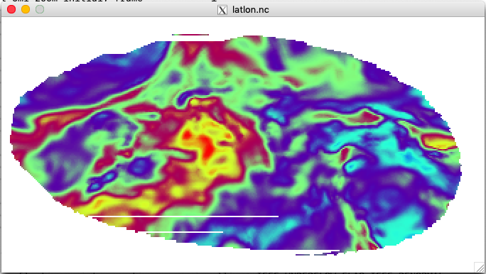
As mentioned in the lectures, the convert_mpas program may produce
some interpolation artifacts as of the time of this tutorial. We expect to have this fixed
in the near future, but for now, we can ignore any interpolation artifacts and animate through
all time slices of several model diagnostic fields in ncview to
gain confidence that our regional simulation is producing plausible results.
After we've taken some time to browse the interpolated diagnostic fields with
ncview, we can make use of NCL to produce figures more suitable
for use in publications or presentations.
In /glade/p/mmm/wmr/mpas_tutorial/ncl_scripts is a template script, regional_cells.ncl,
for plotting the individual cell values from a regional MPAS netCDF file. We can copy this script to our
run directory with the following command:
$ cp /glade/p/mmm/wmr/mpas_tutorial/ncl_scripts/regional_cells.ncl .
By default, this script plots the vegetation type field, ivgtyp, with the view-point
set to 20.0 N latitude, 80.0 E longitude. With the editor of your choice, open
the regional_cells.ncl file and locate the section of the script
with the following (it should be around line 68):
  ;
  ; Center latitude and longitude
  ;
  cenlat = 20.0
  cenlon = 80.0
Let's change the center latitude and longitude values for the view-point to the approximate
center of our regional domain. For our example Mediterranean domain, the following settings
might be reasonable, but if your regional domain is located over a different part of
the globe, you should modify these values as necessary.
  ;
  ; Center latitude and longitude
  ;
  cenlat = 38.0
  cenlon = 20.0
In general, the regional_cells.ncl script reads three environment
variables:
- FNAME - the name of the file containing the field to be plotted
- GNAME - the name of the file containing the mesh information
- T - for time-varying fields, the time period to plot (0 is the first time in a file)
In order to plot the vegetation type field from our initial conditions files, the following
settings of these variables will work:
- FNAME=Mediterranean.init.nc
- GNAME=Mediterranean.init.nc
- T=0
After setting these environment variables and running the NCL script, we should have a plot
equivalent to the one below in a file named "cells.png".
The part of the regional_cells.ncl script that handles the actual plotting
is general enough to handle any field — we just need to set an appropriate plotting range and
color table in the script when changing fields. Next, we can try to modify the script to plot
the precipitable water ("precipw") field using a different color map.
Before proceeding, you may like to open the NCL Color Table Gallery in a new tab to see the available NCL color tables.
With the editor of your choice, open the regional_cells.ncl file and locate
the section of the script (beginning around line 84) where the field to be plotted, the color map, and
the contour levels are set. Let's modify this section of the script so that it looks like the following:
  ;
  ; The field to be plotted
  ;
  h = f->precipw(iTime,:)


  ;
  ; The color map to use
  ; (see https://www.ncl.ucar.edu/Document/Graphics/color_table_gallery.shtml)
  ;
  colormap = "GMT_ocean"

  ;
  ; The number of colors in the color map
  ;
  nColors = 80

  ;
  ; The contour intervals
  ; E.g., fspan(1, 10, 10) yields (/1, 2, 3, 4, 5, 6, 7, 9, 10/)
  ; Typically, we have nColors-1 levels
  ;
  cnLevels = fspan(0.0, 50.0, nColors-1)
We located the "GMT_ocean" color table from the NCL Color Table Gallery link, above. Before re-running
the script, we will need to set the FNAME environment variable to the name
of one of our diagnostics model output files. If our regional simulation has progressed through at least
forecast hour 24, we could use the following:
$ export FNAME=diag.2019-09-02_00.00.00.nc
We can then re-run the script to produce a plot like the one below.
With the remaining time in this session, feel free to experiment with plotting other fields from
any of the netCDF output files. Browsing the model output that has been converted to a latitude-longitude
grid with the convert_mpas before deciding on the field to plot and the range
of values to set in the regional_cells.ncl script may be helpful.
In this section, we'll restart a simulation from the end of the five-day, global 240-km
simulation that we started in the second section. Before restarting the simulation, though,
we'll define new output streams.
Optionally, before restarting the simulation, we can also try adding a list of sounding
locations for the simulation.
After launching the restart simulation with new output streams (and perhaps some sounding
output), we'll practice using some NCL scripts to visualize the first five days of output
from the variable-resolution 240-km – 48-km simulation
As we saw in the lectures, setting up a simulation to restart from a previously
run simulation is relatively simple. We'll begin by making sure that we're in
the directory where we ran the original, 5-day 240-km global simulation:
$ cd /glade/scratch/${USER}/mpas_tutorial/240km_uniform
Before making any changes to the namelist.atmosphere file,
we will first check to see which restart files are available; if our original simulation
completed successfully, we should have one restart file per day, valid at the end of
each of the five days of the simulation:
$ ls -l restart*nc
-rw-r--r-- 1 duda ncar 197382136 Apr  8 23:57 restart.2014-09-11_00.00.00.nc
-rw-r--r-- 1 duda ncar 197382136 Apr  8 23:57 restart.2014-09-12_00.00.00.nc
-rw-r--r-- 1 duda ncar 197382136 Apr  8 23:58 restart.2014-09-13_00.00.00.nc
-rw-r--r-- 1 duda ncar 197382136 Apr  8 23:59 restart.2014-09-14_00.00.00.nc
-rw-r--r-- 1 duda ncar 197382136 Apr  8 23:59 restart.2014-09-15_00.00.00.nc
In principle, we could restart our simulation from any of these files, but we'll begin
from the last available file, valid at 0000 UTC on 15 September.
There are just two changes that need to be made to the namelist.atmosphere
file: we need to set the starting time of the simulation to 2014-09-15_00:00:00
and we need to set the config_do_restart option to true:
&nhyd_model
    config_start_time = '2014-09-15_00:00:00'
/
&restart
    config_do_restart = true
/
We can keep all of the other namelist options as they were, including the config_run_duration
option — restarting the simulation and running for another five days should be fine, since we had a total
of 10 days of SST and sea-ice information in our surface update file.
Before running the model, we'll make a few other changes as described in the next sections!
We may also like to write out some additional fields from our restart simulation at a higher
temporal frequency. You may recall from the lectures that we can define new output streams
in the streams.atmosphere file.
We will provide an example here of writing out the 10-meter AGL horizontal winds every 60 minutes,
but you can feel free to look through Appendix D of the MPAS-Atmosphere Users' Guide to see
if there are any other fields that you may like to write out.
Let's define a new output stream named "sfc_winds" in the streams.atmosphere file:
<stream name="sfc_winds"
        type="output"
        filename_template="surface_winds.$Y-$M-$D_$h.nc"
        filename_interval="output_interval"
        output_interval="60:00" >

        <var name="u10"/>
        <var name="v10"/>
</stream>
This new stream must be defined somewhere between the opening <streams>
and closing </streams> tags in the streams.atmosphere file.
Note in the stream definition above that the files that will be written will have names like
surface_winds.2014-09-15_00.nc, surface_winds.2014-09-15_01.nc,
etc. by our choice of the "filename_template". Also, MPAS will create new files at each output time, rather than
packing many time records into the same file; this is controlled by the "filename_interval" option. Finally, note
that the stream will be written every 60 minutes. Since our simulation starts at 00:00:00 UTC, the minutes and seconds
part of the output files is unnecessary. Of course, we may want to add $m and
$s to our filename template if we were writing this stream more frequently than once
per hour.
In the next section, we'll describe the steps to write out vertical profiles at specific (lat,lon) locations
before we run our restart simulation.
It may at times also be helpful to write out vertical profiles of basic model fields
at specified (lat,lon) locations from a model simulation. In MPAS terminology, this
is described as writing "soundings" from the simulation.
In principle, we can write out soundings for as many locations as we would like.
Here, we'll describe how to write out soundings from three locations: Boulder, Colorado;
McMurdo Station, Antarctica; and New Delhi, India.
We will need to specify the locations for the soundings in a text file named sounding_locations.txt
in our model run directory:
40.0   -105.25  Boulder
28.7     77.2   NewDelhi
-77.85  166.67  McMurdo
The three columns of the file contain the latitude, longitude, and name of the sounding. The latitude and longitude
are given as decimal degrees, and the name cannot contain whitespace (since it will be used to name output files).
For this exercise, if you would prefer to write out soundings for different locations,
feel free to change the list of locations as you would like!
Lastly, we need to specify how frequently these soundings will be written during the model simulation. This is
done through the config_sounding_interval option in the namelist.atmosphere
file. By default, this option can be found near the bottom of the file. Let's choose to write soundings every
three hours:
&soundings
    config_sounding_interval = '3:00:00'
/
Having set the output interval for soundings, we're ready to make a restart simulation.
Now that we've edited our namelist.atmosphere file for our restart
run, we've added a new output stream with surface winds to the streams.atmosphere
file, and we've specified a list of locations for which profiles will be written every three hours,
we can restart the model and simulate an additional five days
by submitting our existing run_model.pbs
script with qsub:
$ qsub run_model.pbs
Once the job has started to run, it's a good idea to check several points:
- Does running tail -f log.atmosphere.0000.out show timesteps being taken by the model?
- Do you see new output files named surface_winds.2014-09-15_00.nc, etc.?
- Do you see sounding files for Boulder, New Delhi, and McMurdo Station as files with the .snd suffix?
If all of the above check out, our restart simulation is successfully running! In the next section, we'll look
at a couple of new NCL scripts for plotting model output.
Now that our restart simulation is running, we can examine in more detail an example NCL script
for plotting horizontal fields as individual cells. To try out this script, we can work with
output from our 240km – 48km variable-resolution simulation.
In order to plot horizontal fields, we can begin by ensuring that we are in
the 240-48km_variable directory before copying over
the latlon_cells.ncl script:
$ cd /glade/scratch/${USER}/mpas_tutorial/240-48km_variable
$ cp /glade/p/mmm/wmr/mpas_tutorial/ncl_scripts/latlon_cells.ncl .
This script reads the name of the MPAS NetCDF file with SCVT mesh information from an
environment variable named GNAME (roughly, "G" means "grid").
The MPAS NetCDF file that contains the actual field to be plotted is identified by
the environment variable FNAME (roughly, "F" means "field").
We'll plot a field from the diag.2014-09-11_00.00.00.nc file.
The mesh information can be found in the MPAS initial conditions file, which may be named
SouthAmerica.init.nc, though you may have chosen a different
name corresponding to a different location of refinement. We'll set the GNAME
and FNAME environment variables before proceeding:
$ export GNAME=SouthAmerica.init.nc
$ export FNAME=diag.2014-09-11_00.00.00.nc
Remember, your initial conditions file may have a different name!
By default, the latlon_cells.ncl script plots the lowest-model-level
wind speed, and the output is saved to a PNG image in a file named cell_plot.png.
Running the script should produce this plot, which you can view with the display command.
$ ncl latlon_cells.ncl
$ display cell_plot.png
Since we are working with a variable-resolution mesh, we may like to set a plotting window to cover
only part of the refined region in our simulation. We can set a plotting window in the latlon_cells.ncl
script by editing the section of the script that looks like this:
; The bounding box for the plot
mapLeft   = -180.0
mapRight  = 180.0
mapBottom = -90.0
mapTop    =  90.0
Feel free to set the plotting window however you would like for your variable-resolution simulation. For example,
if we were to set the plotting window to cover South America before re-running the script, the result might look
like the following:
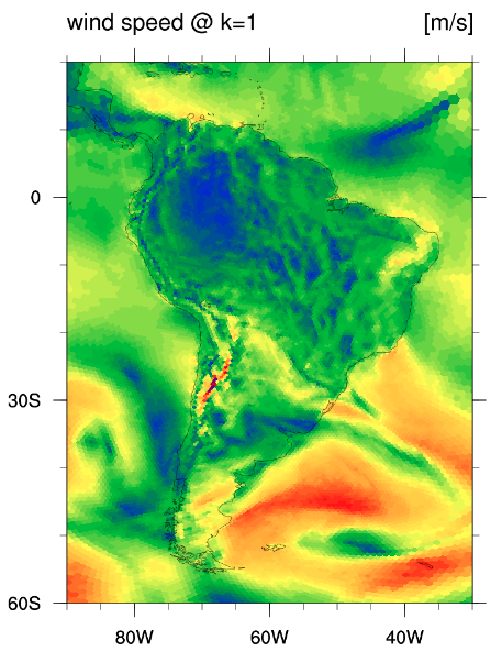
Finally, we may like to plot other fields. We can see which fields were written to
the diag.*.nc files using ncdump:
$ ncdump -h diag.2014-09-11_00.00.00.nc
If, for example, we would like to plot Convective Available Potential Energy (CAPE), we could
edit the latlon_cells.ncl script near the comment "The field to be plotted"
so that it looked like the following:
; The field to be plotted
h   = f->cape(0,:)

; The field name
field_name = "CAPE"
field_units = "[J/kg]"

; The range of field values to plot (start, stop, number)
cnLevels = fspan(0,3000,50)
Generally, we will need to assign the variable to be plotted, specify the plotting name and units
for the field, and specify a range of value for the field. Making these changes and re-running
the NCL script might produce a plot like the following:
Now that you have a feel for how to edit the latlon_cells.ncl script,
feel free to try plotting other fields!
In this section, we'll get some experience in making source-code changes to add
a passive tracer to the model. Although the exercises in this section are independent
of those in other section, it may be best to finish the exercises from the previous
section first, since we will be changing the model source code and re-compiling
the model executable.
We'll begin by defining our new passive tracer in the Registry.xml
file for the init_atmosphere core. Let's change directories to
the copy of the MPAS-Model source code in our /glade/scratch/${USER}/mpas_tutorial directory:
$ cd /glade/scratch/${USER}/mpas_tutorial/MPAS-Model
Opening up the src/core_init_atmosphere/Registry.xml file with
our editor of choice, we will look for the var_array section
named "scalars"; it should look something like this:
                <var_array name="scalars" type="real" dimensions="nVertLevels nCells Time">
                        <var name="qv" array_group="moist" units="kg kg^{-1}"
                             description="Water vapor mixing ratio"/>

                        <var name="qc" array_group="moist" units="kg kg^{-1}"
                             description="Cloud water mixing ratio"/>

                        <var name="qr" array_group="moist" units="kg kg^{-1}"
                             description="Rain water mixing ratio"/>
                </var_array>
As we saw in the lectures, we will need to add our new passive tracers here. Let's add a new
passive tracer named "mytracer1". The array_group that we assign to
this tracer can be anything other than "moist". By convention, we'll
call the array group for this new tracer "passive". After adding our
new tracer, the "scalars" var_array should
look like this:
                <var_array name="scalars" type="real" dimensions="nVertLevels nCells Time">
                        <var name="qv" array_group="moist" units="kg kg^{-1}"
                             description="Water vapor mixing ratio"/>

                        <var name="qc" array_group="moist" units="kg kg^{-1}"
                             description="Cloud water mixing ratio"/>

                        <var name="qr" array_group="moist" units="kg kg^{-1}"
                             description="Rain water mixing ratio"/>

                        <var name="mytracer1" array_group="passive" units="kg kg^{-1}"
                             description="A simple passive tracer"/>
                </var_array>
After making this change to the Registry.xml file, we'll clean and re-compile the init_atmosphere core.
Recall that, after we make changes to the Registry.xml file, we need to "clean" the build first so that
the changes take effect. Later, when we modify only Fortran source code, there will be no need to "clean"
before re-compiling. The following two commands should suffice:
$ make clean CORE=init_atmosphere
$ qcmd -A UMMM0004 -- make -j4 gfortran CORE=init_atmosphere PRECISION=single
If compilation was successful, we should now have a new init_atmosphere_model
executable. At this point, if we were to create new initial conditions, the "mytracer1" field would be
present in the initial conditions, but it would be zero everywhere. We next need to add code to define
the initial conditions for "mytracer1".
To define the initial value of our new tracer, use your preferred editor to open the src/core_init_atmosphere/mpas_init_atm_cases.F file. Search for these two lines of code that call the routine to initialize real-data test cases:
             call init_atm_case_gfs(block_ptr, mesh, nCells, nEdges, nVertLevels, fg, state, &
                                    diag, diag_physics, config_init_case, block_ptr % dimensions, block_ptr % configs)
An appropriate place to add a call to our tracer initialization routine would be directly after the call
to init_atm_case_gfs. Let's add a new line of code below this to call a new subroutine,
which we'll name init_tracers.
             call init_atm_case_gfs(block_ptr, mesh, nCells, nEdges, nVertLevels, fg, state, &
                                    diag, diag_physics, config_init_case, block_ptr % dimensions, block_ptr % configs)
             call init_tracers(mesh, state)
Notice that this new routine (which we have yet to define!) takes as input two arguments; as we will see, these
two arguments are MPAS "pools", which we discussed in the lectures.
As a start, we will define the init_tracers function so that it simply writes a message
to the log file. At the bottom of the src/core_init_atmosphere/mpas_init_atm_cases.F,
but before the line "end module init_atm_cases", let's add the following Fortran code:
   subroutine init_tracers(mesh, state)

       implicit none

       type (mpas_pool_type), intent(in) :: mesh
       type (mpas_pool_type), intent(inout) :: state

       call mpas_log_write('====== Handling tracer initialization ======')

   end subroutine init_tracers
After saving our code changes, we can re-compile the init_atmosphere core with:
$ qcmd -A UMMM0004 -- make -j4 gfortran CORE=init_atmosphere PRECISION=single
Again, because we have not changed the Registry.xml file since we last re-compiled,
there's no need to "make clean".
Compilation should take just a minute, and if it completes successfully, we're ready to try out our modified
code, even though it won't actually create initial conditions for our passive tracer, yet. So that we don't
overwrite files from any of our previous sessions, we'll work in a new directory, passive_tracer:
$ cd /glade/scratch/${USER}/mpas_tutorial
$ mkdir passive_tracer
$ cd passive_tracer
We'll test out our passive tracer on the 240-km uniform mesh, for which we have already created a "static" file.
Now that we have experience in creating initial conditions, the following procedure should seem familiar:
$ ln -s /glade/scratch/${USER}/mpas_tutorial/240km_uniform/x1.10242.static.nc .
$ ln -s /glade/p/mmm/wmr/mpas_tutorial/met_data/ERA5:2014-09-10_00 .
$ ln -s /glade/scratch/${USER}/mpas_tutorial/MPAS-Model/init_atmosphere_model .
$ cp /glade/scratch/${USER}/mpas_tutorial/MPAS-Model/namelist.init_atmosphere .
$ cp /glade/scratch/${USER}/mpas_tutorial/MPAS-Model/streams.init_atmosphere .
As in Section 2.1, we'll edit the namelist.init_atmosphere so that it looks
like the following:
&nhyd_model
    config_init_case = 7
    config_start_time = '2014-09-10_00:00:00'
/
&dimensions
    config_nvertlevels = 41
    config_nsoillevels = 4
    config_nfglevels = 38
    config_nfgsoillevels = 4
/
&data_sources
    config_met_prefix = 'ERA5'
    config_use_spechumd = false
/
&vertical_grid
    config_ztop = 30000.0
    config_nsmterrain = 1
    config_smooth_surfaces = true
    config_dzmin = 0.3
    config_nsm = 30
    config_tc_vertical_grid = true
    config_blend_bdy_terrain = false
/
&interpolation_control
    config_extrap_airtemp = 'lapse-rate'
/
&preproc_stages
    config_static_interp = false
    config_native_gwd_static = false
    config_vertical_grid = true
    config_met_interp = true
    config_input_sst = false
    config_frac_seaice = true
/
We'll then edit the filename that will be read by the "input" stream in
the streams.init_atmosphere file so that it matches the
name of our "static" file:
<immutable_stream name="input"
                  type="input"
                  filename_template="x1.10242.static.nc"
                  input_interval="initial_only"/>
Also as in Section 2.1, we'll change the name of the initial conditions file to be created:
<immutable_stream name="output"
                  type="output"
                  filename_template="x1.10242.init.nc"
                  packages="initial_conds"
                  output_interval="initial_only" />
We should now be able to run the init_atmosphere_model executable
to produce an x1.10242.init.nc file:
$ qcmd -A UMMM0004 -- ./init_atmosphere_model
If there were no errors in the log.init_atmosphere.0000.out file, we can check for the presence
of our passive tracer in the x1.10242.init.nc file:
$ ncdump -h x1.10242.init.nc | grep mytracer1
Besides the creation of the x1.10242.init.nc file, we should also look for this message in the log.init_atmosphere.0000.out file:
====== Handling tracer initialization ======
If all was successful, we can go back to the MPAS-Model directory and add code to provide
initial conditions for our passive tracer. Let's change back to the MPAS source code directory:
$ cd /glade/scratch/${USER}/mpas_tutorial/MPAS-Model
Using our favorite editor, let's open the src/core_init_atmosphere/mpas_init_atm_cases.F file and
change the code for our init_tracers subroutine so that it looks like the following:
   subroutine init_tracers(mesh, state)

       implicit none

       type (mpas_pool_type), intent(in) :: mesh
       type (mpas_pool_type), intent(inout) :: state

       integer, pointer :: index_mytracer1
       integer, pointer :: nCells
       integer, pointer :: nVertLevels

       integer :: k, iCell

       real (kind=RKIND), dimension(:), pointer :: latCell
       real (kind=RKIND), dimension(:), pointer :: lonCell
       real (kind=RKIND), dimension(:,:,:), pointer :: scalars

       call mpas_log_write('====== Handling tracer initialization ======')

       call mpas_pool_get_dimension(mesh, 'nCells', nCells)
       call mpas_pool_get_dimension(mesh, 'nVertLevels', nVertLevels)

       call mpas_pool_get_dimension(state, 'index_mytracer1', index_mytracer1)

       call mpas_pool_get_array(state, 'scalars', scalars)
       call mpas_pool_get_array(mesh, 'latCell', latCell)
       call mpas_pool_get_array(mesh, 'lonCell', lonCell)

       do iCell = 1, nCells
           do k = 1, nVertLevels
               scalars(index_mytracer1,k,iCell) = &
                         0.0001 * 0.5 * (sin(latCell(iCell)*4.0) * &
                                         sin(lonCell(iCell)*8.0) + 1.0)
           end do
       end do

   end subroutine init_tracers
Based on what was discussed in the MPAS software lecture about Registry, pools, and logging,
you have the necessary information at your disposal to make sense of the code for the
init_tracers routine!
After saving our changes, we can re-compile the init_atmosphere core once again:
$ qcmd -A UMMM0004 -- make -j4 gfortran CORE=init_atmosphere PRECISION=single
We can now try creating new initial conditions with our updated init_tracers routine.
Let's change back to the passive_tracer directory, remove the old
x1.10242.init.nc file, and create a new initial conditions file:
$ cd /glade/scratch/${USER}/mpas_tutorial/passive_tracer
$ rm x1.10242.init.nc
$ qcmd -A UMMM0004 -- ./init_atmosphere_model
If the creation of the new x1.10242.init.nc file was successful, you may like to try
using the convert_mpas utility to see what our new "mytracer1" field looks like. For
a quick reminder of how the convert_mpas tool works, you may find it helpful to refer
back to Section 3.3.
Now that we have a new passive tracer in our initial conditions, we'll need to edit
the Registry.xml file for the atmosphere
core so that the model itself will know about the new tracer.
Let's begin by changing back to the model source code directory:
$ cd /glade/scratch/${USER}/mpas_tutorial/MPAS-Model
We can edit the src/core_atmosphere/Registry.xml file, recalling from
the lectures that we not only need to define the tracer, but we also need to define an array
that will hold the tendencies for the tracer. Even if we don't supply any sources or sinks,
the model needs memory to be allocated for the tracer tendency, e.g., for use in the scalar
transport routines.
In the src/core_atmosphere/Registry.xml file, search for the word "var_array"
several times until you come to the definition of the scalars var_array
tag, which should begin with lines that look like this:
<var_array name="scalars" type="real" dimensions="nVertLevels nCells Time">
        <var name="qv" array_group="moist" units="kg kg^{-1}"
             description="Water vapor mixing ratio"/>
Let's add a new XML var tag inside the var_array
tag to define our new "mytracer1" tracer; this new tag may look something like the following:
        <var name="mytracer1" array_group="passive" units="kg kg^{-1}"
             description="Our first passive tracer"/>
Remember: it's important that the passive tracer belongs to an array_group
other than "moist"; here, we've just used the string "passive", though in principle you could choose
another name.
Similarly, we need to define a tendency array for our new passive tracer. Searching for the word "scalars_tend",
we should find a section of XML for the scalars_tend var_array
that begins with the following lines:
<!-- scalar tendencies -->
<var_array name="scalars_tend" type="real" dimensions="nVertLevels nCells Time">
        <var name="tend_qv" name_in_code="qv" array_group="moist" units="kg m^{-3} s^{-1}"
             description="Tendency of water vapor mass per unit volume divided by d(zeta)/dz"/>
We'll define a new var entry in this var_array for our
passive tracer tendency; this new entry might look something like the following:
        <var name="tend_mytracer1" name_in_code="mytracer1" array_group="passive" units="kg m^{-3} s^{-1}"
             description="Tendency of our first tracer mass per unit volume divided by d(zeta)/dz"/>
Don't forget to set the value for array_group to "passive"!
With these changes to the Registry.xml file, we can re-compile the atmosphere
core. But, we'll first need to "clean" the code, since the last core that we compiled was the init_atmosphere core.
$ make clean CORE=atmosphere
$ qcmd -A UMMM0004 -- make -j4 gfortran CORE=atmosphere PRECISION=single
If compilation was successful, we can change directories to our passive_tracer directory and
prepare to run MPAS:
$ cd /glade/scratch/${USER}/mpas_tutorial/passive_tracer
You may recall from Section 2.3 that we need the MPAS executable, atmosphere_model, as well as
a number other files in order to run a simulation. Let's link or copy these files as we did in Section 2.3:
$ ln -s /glade/scratch/${USER}/mpas_tutorial/MPAS-Model/atmosphere_model .
$ cp /glade/scratch/${USER}/mpas_tutorial/MPAS-Model/namelist.atmosphere .
$ cp /glade/scratch/${USER}/mpas_tutorial/MPAS-Model/streams.atmosphere .
$ cp /glade/scratch/${USER}/mpas_tutorial/MPAS-Model/stream_list.atmosphere.* .
$ ln -s /glade/scratch/${USER}/mpas_tutorial/MPAS-Model/src/core_atmosphere/physics/physics_wrf/files/* .
Now, we can proceed to set up the namelist.atmosphere and
streams.atmosphere files as we did in Section 2.3 before running the model
simulation. In order to run the model in parallel with 36 MPI tasks, we'll need to link
the /glade/p/mmm/wmr/mpas_tutorial/meshes/x1.10242.graph.info.part.36 mesh partition file into our
working directory:
$ ln -s /glade/p/mmm/wmr/mpas_tutorial/meshes/x1.10242.graph.info.part.36 .
When running the model, we can copy the run_model.pbs batch script
before submitting the job with qsub:
$ cp /glade/p/mmm/wmr/mpas_tutorial/job_scripts/run_model.pbs .
$ qsub run_model.pbs
The entire set of scalars is written to the default "history" files, so as soon as the first several
output files are available, we can try making plots of our new "mytracer1" passive tracer. Then, we can stop
the model simulation and proceed to the next sub-section, where we will add sources and sinks for our new tracer
before running a longer simulation.
To terminate a running job on Cheyenne, we first need to find its job ID from qstat:
$ qstat -u $USER

chadmin1.ib0.cheyenne.ucar.edu:
                                                            Req'd  Req'd   Elap
Job ID          Username Queue    Jobname    SessID NDS TSK Memory Time  S Time
--------------- -------- -------- ---------- ------ --- --- ------ ----- - -----
7544900.chadmin duda     regular  atmosphere  59452   1  36    --  01:00 R 00:01
We just need the numeric part of the job ID in order to cancel the job with qdel:
$ qdel 7544900
You can verify that the job has been terminated by waiting a minute or so before running qstat again.
Having added a passive tracer to our initial conditions and defined the tracer in the model
so that it will be transported during a simulation, it's not much additional work to define sources
and sinks for the tracer. Here, we will define time-invariant sources and sinks that are
set up when the model begins running, but we could in principle define time-varying sources
and sinks that are periodically updated from an input file, for example.
To add time-invariant sources and sinks, we can change to our MPAS-Model source directory
and edit the src/core_atmosphere/Registry.xml file with the editor
of our choice. Searching for the section of the file that begins the definition of
the "tend" var_struct around line 1781 we should see the following:
        <var_struct name="tend" time_levs="1">


                <!-- tendencies for prognostic variables -->
Just below the tendencies for prognostic variables comment line,
let's add a definition for our passive tracer's sources/sinks:
                <var name="mytracer1_sources" type="real"
                     dimensions="nVertLevels nCells Time"
                     units="kg m^{-2} s^{-1}"
                     description="Our first passive tracer areal production rate" />
As in the lecture on adding passive tracers, our example tracer will be produced and destroyed
at the surface of the model.
Next, we can add code to set the "mytracer1_sources" field when the model starts up. In
the src/core_atmosphere/mpas_atm_core.F source file in
the atm_mpas_init_block subroutine (around line 355), we will add declarations
of two new array pointers at the end of the variable declarations as in the highlighted code, below:
      integer, pointer :: nThreads
      integer, dimension(:), pointer :: cellThreadStart, cellThreadEnd
      integer, dimension(:), pointer :: cellSolveThreadStart, cellSolveThreadEnd
      integer, dimension(:), pointer :: edgeThreadStart, edgeThreadEnd
      integer, dimension(:), pointer :: edgeSolveThreadStart, edgeSolveThreadEnd
      integer, dimension(:), pointer :: vertexThreadStart, vertexThreadEnd
      integer, dimension(:), pointer :: vertexSolveThreadStart, vertexSolveThreadEnd


      logical, pointer :: config_do_restart, config_do_DAcycling

      real (kind=RKIND), dimension(:,:), pointer :: mytracer1_sources
      integer, dimension(:), pointer :: ivgtyp

      call atm_compute_signs(mesh)
Then, near the end of the atm_mpas_init_block subroutine, we can add
code to set the production/destruction of our tracer based on whether a model cell is land or water:
      call mpas_pool_get_array(tend, 'mytracer1_sources', mytracer1_sources)
      call mpas_pool_get_array(sfc_input, 'ivgtyp', ivgtyp)

      mytracer1_sources(:,:) = 0.0_RKIND
      do iCell=1,nCells
         ! Assume that vegetation category 17 is water
         ! (true for MODIS land use, not true for USGS)
         if (ivgtyp(iCell) == 17) then
            ! 2 g/m^2/day destruction over water
            mytracer1_sources(1,iCell) = -0.002 / 86400.0
         else
            ! 4 g/m^2/day production over land
            mytracer1_sources(1,iCell) = 0.004 / 86400.0
         end if
      end do

   end subroutine atm_mpas_init_block
Finally, we can add our source terms to the tendency array for our new tracer.
In src/core_atmosphere/physics/mpas_atmphys_todynamics.F at the bottom of
the variable declarations in the physics_get_tend subroutine,
we can add the following variable declarations around line 124:
  real(kind=RKIND),dimension(:,:),allocatable:: theta,tend_th

 integer, pointer :: index_mytracer1
 real(kind=RKIND),dimension(:,:),pointer:: mytracer1_sources
 real(kind=RKIND),dimension(:,:),pointer:: zz
 real(kind=RKIND),dimension(:,:),pointer:: zgrid

 !========================================================================================================
  call mpas_pool_get_dimension(mesh, 'nCells', nCells)
Then, near the bottom of the subroutine before several arrays are deallocated, we can add code
to include our source terms in the tendency for our passive tracer:
 call mpas_pool_get_dimension(state, 'index_mytracer1', index_mytracer1)
 call mpas_pool_get_array(tend, 'mytracer1_sources', mytracer1_sources)
 call mpas_pool_get_array(mesh, 'zz', zz)
 call mpas_pool_get_array(mesh, 'zgrid', zgrid)

 do i = 1, nCellsSolve
    do k = 1, nVertLevels
       tend_scalars(index_mytracer1,k,i) = tend_scalars(index_mytracer1,k,i) &
            + mytracer1_sources(k,i) / (zgrid(k+1,i) - zgrid(k,i)) / zz(k,i)
    end do
 end do

 !
 ! Clean up any pointers that were allocated with zero size before the call to
 ! physics_get_tend_work
 !
Since we have modified the Registry.xml file, we will need to clean the code
before re-compiling the model:
$ make clean CORE=atmosphere
$ qcmd -A UMMM0004 -- make -j4 gfortran CORE=atmosphere PRECISION=single
After the model has been successfully re-compiled, we can change directories to our run directory,
remove any existing model output files, and re-run the model:
$ cd /glade/scratch/${USER}/mpas_tutorial/passive_tracer
$ rm -f diag*nc history*nc
$ qsub run_model.pbs
Once the model has started to run and has produced several history files — which should now
contain our new "mytracer1" field — we can use, e.g., convert_mpas
to interpolate the model history files to a lat-lon grid for quick visualization of our new tracer
with sources and sinks in the lowest model layer!
In this final section, we will add a new diagnostic field to the model: an approximation
to the radiative energy balance computed as the integrated difference between the outgoing
and incoming radiation fluxes (both long-wave and short-wave) at the top of the model.
The integration will occur between output times of the new diagnostic field.
Disclaimer: this exercise was developed by a software engineer; if the diagnostic
described here makes no physical sense or otherwise contains errors, please don't let
this negatively affect your views of MPAS-Atmosphere as a scientifically credible model!
The MPAS-Atmosphere model contains a framework for organizing new diagnostic computations
into their own modules, which contain routines to perform different stages of the computation
of the diagnostic (e.g, accumulation, averaging, and resetting). To separate the complications
of computing the diagnostic from those of implementing the diagnostic in the MPAS-Atmosphere
code, we can begin by simply defining a variable for our new energy balance diagnostic along
with some placeholder code with print statements. We can then verify that the model compiles
correctly and prints the expected lines to the log.atmosphere.0000.out
file, demonstrating that at a technical level we have successfully connected our new diagnostic
module with the MPAS-Atmosphere diagnostic framework. In the next section, then, we will be
free to focus on the correct computation of the diagnostic itself.
Let's begin by changing to the directory containing our MPAS-Model source code:
$ cd /glade/scratch/${USER}/mpas_tutorial/MPAS-Model
All of the changes for our energy balance diagnostic will be confined to the src/core_atmosphere/diagnostics
subdirectory; we can change to that sub-directory now:
$ cd src/core_atmosphere/diagnostics
There are just three files in this directory that serve as the interface between the rest of the MPAS-Atmosphere model
and our new diagnostic:
- Makefile — changes here will ensure that our new Fortran code
will be used when we recompile MPAS
- Registry_diagnostics.xml — changes here will allow any new
variables defined by our diagnostic code to be available to the rest of the MPAS code (in
particular, to the stream manager, which allows our diagnostic field to be written to output
files)
- mpas_atm_diagnostics_manager.F — changes here will ensure that
the different stages of computation required by our new diagnostic are called at the correct
points in each model timestep
Before modifying the three files listed above, we can first define a new variable in an XML file for our diagnostic. With the editor of your
choice, create a new file named Registry_energy_balance.xml with the following contents (click the light blue header):
<!-- ******************************* -->
<!-- Energy balance diagnostics      -->
<!-- ******************************* -->

<var_struct name="diag" time_levs="1">

        <var name="accradflux" type="real" dimensions="nCells Time" units="J m^{-2}"
             description="Accumulated net radiative energy flux at the top of the atmosphere"/>

</var_struct>
We can also create a new Fortran module with place-holder code, in which each subroutine simply prints a message to the log file. With
the editor of your choice, create a new file named energy_balance_diagnostics.F with the following contents
(click the light blue header):
module energy_balance

    use mpas_derived_types, only : MPAS_pool_type, MPAS_clock_type
    use mpas_kind_types, only : RKIND
    use mpas_log, only : mpas_log_write

    type (MPAS_clock_type), pointer :: clock

    real(kind=RKIND), dimension(:), pointer :: accradflux
    real(kind=RKIND), dimension(:), pointer :: lwdnt
    real(kind=RKIND), dimension(:), pointer :: lwupt
    real(kind=RKIND), dimension(:), pointer :: swdnt
    real(kind=RKIND), dimension(:), pointer :: swupt

    public :: energy_balance_setup, &
              energy_balance_update, &
              energy_balance_compute, &
              energy_balance_reset, &
              energy_balance_cleanup

    private


    contains


    subroutine energy_balance_setup(configs, all_pools, simulation_clock)

        use mpas_derived_types, only : MPAS_pool_type, MPAS_clock_type
        use mpas_pool_routines, only : mpas_pool_get_subpool, mpas_pool_get_array

        implicit none

        type (MPAS_pool_type), pointer :: configs
        type (MPAS_pool_type), pointer :: all_pools
        type (MPAS_clock_type), pointer :: simulation_clock

        type (MPAS_pool_type), pointer :: diag
        type (MPAS_pool_type), pointer :: diag_physics

        clock => simulation_clock

        call mpas_pool_get_subpool(all_pools, 'diag', diag)
        call mpas_pool_get_subpool(all_pools, 'diag_physics', diag_physics)

        !
        ! Save pointers to all fields that will be used in the computation of
        ! the energy balance diagnostic
        !
        call mpas_pool_get_array(diag, 'accradflux', accradflux)
        call mpas_pool_get_array(diag_physics, 'lwdnt', lwdnt)
        call mpas_pool_get_array(diag_physics, 'lwupt', lwupt)
        call mpas_pool_get_array(diag_physics, 'swdnt', swdnt)
        call mpas_pool_get_array(diag_physics, 'swupt', swupt)

        call mpas_log_write('TESTING: energy_balance_setup')

    end subroutine energy_balance_setup


    subroutine energy_balance_update()

        implicit none

        call mpas_log_write('TESTING: energy_balance_update')

    end subroutine energy_balance_update


    subroutine energy_balance_compute()

        implicit none

        call mpas_log_write('TESTING: energy_balance_compute')

    end subroutine energy_balance_compute


    subroutine energy_balance_reset()

        implicit none

        call mpas_log_write('TESTING: energy_balance_reset')

    end subroutine energy_balance_reset


    subroutine energy_balance_cleanup()

        implicit none

        call mpas_log_write('TESTING: energy_balance_cleanup')

    end subroutine energy_balance_cleanup

end module energy_balance
Having defined a variable to store our diagnostic as well as placeholder code in a new Fortran module, we can edit the Makefile,
Registry_diagnostics.xml, and mpas_atm_diagnostics_manager.F files to connect our diagnostic.
The required changes to each of these files are highlighted in the code, below.
.SUFFIXES: .F .o

#
# Add new diagnostic modules to DIAGNOSTIC_MODULES
#
DIAGNOSTIC_MODULES = \
	mpas_atm_diagnostic_template.o \
	isobaric_diagnostics.o \
	convective_diagnostics.o \
	pv_diagnostics.o \
	soundings.o \
	energy_balance_diagnostics.o

isobaric_diagnostics.o: mpas_atm_diagnostics_utils.o

convective_diagnostics.o: mpas_atm_diagnostics_utils.o

pv_diagnostics.o: mpas_atm_diagnostics_utils.o

energy_balance_diagnostics.o: mpas_atm_diagnostics_utils.o

soundings.o:


################### Generally no need to modify below here ###################


OBJS = mpas_atm_diagnostics_manager.o mpas_atm_diagnostics_utils.o

all: $(DIAGNOSTIC_MODULS) $(OBJS)

mpas_atm_diagnostics_manager.o: mpas_atm_diagnostics_utils.o $(DIAGNOSTIC_MODULES)


clean:
	$(RM) *.o *.mod *.f90
	@# Some Intel compilers generate *.i files; clean them up, too
	$(RM) *.i

.F.o:
	$(RM) $@ $*.mod
ifeq "$(GEN_F90)" "true"
	$(CPP) $(CPPFLAGS) $(PHYSICS) $(CPPINCLUDES) $< > $*.f90
	$(FC) $(FFLAGS) -c $*.f90 $(FCINCLUDES) -I../../framework -I../../operators -I../dynamics -I../physics -I../physics/physics_wrf -I../../external/esmf_time_f90
else
	$(FC) $(CPPFLAGS) $(PHYSICS) $(FFLAGS) -c $*.F $(CPPINCLUDES) $(FCINCLUDES) -I../../framework -I../../operators -I../dynamics -I../physics -I../physics/physics_wrf -I../../external/esmf_time_f90
endif
<!-- ******************************* -->
<!-- Begin includes from diagnostics -->
<!-- ******************************* -->

#include "Registry_template.xml"

<!-- isobaric diagnostics -->
#include "Registry_isobaric.xml"

<!-- convective diagnostics -->
#include "Registry_convective.xml"

<!-- PV diagnostics -->
#include "Registry_pv.xml"

<!-- soundings -->
#include "Registry_soundings.xml"

<!-- energy balance -->
#include "Registry_energy_balance.xml"

<!-- ******************************* -->
<!-- End includes from diagnostics -->
<!-- ******************************* -->
! Copyright (c) 2016,  Los Alamos National Security, LLC (LANS)
! and the University Corporation for Atmospheric Research (UCAR).
!
! Unless noted otherwise source code is licensed under the BSD license.
! Additional copyright and license information can be found in the LICENSE file
! distributed with this code, or at http://mpas-dev.github.com/license.html
!
module mpas_atm_diagnostics_manager

    private

    public :: mpas_atm_diag_setup, &
              mpas_atm_diag_update, &
              mpas_atm_diag_compute, &
              mpas_atm_diag_reset, &
              mpas_atm_diag_cleanup

    contains


    !-----------------------------------------------------------------------
    !  routine MPAS_atm_diag_setup
    !
    !> \brief Initialize the diagnostics manager and all diagnostics
    !> \author Michael Duda
    !> \date   6 September 2016
    !> \details
    !>  Initialize the diagnostics manager and all diagnostics.
    !
    !-----------------------------------------------------------------------
    subroutine mpas_atm_diag_setup(stream_mgr, configs, structs, clock, dminfo)

        use mpas_atm_diagnostics_utils, only : mpas_atm_diag_utils_init
        use mpas_derived_types, only : MPAS_streamManager_type, MPAS_pool_type, MPAS_clock_type, dm_info
        use diagnostic_template, only : diagnostic_template_setup
        use isobaric_diagnostics, only : isobaric_diagnostics_setup
        use convective_diagnostics, only : convective_diagnostics_setup
        use pv_diagnostics, only : pv_diagnostics_setup
        use soundings, only : soundings_setup
        use energy_balance, only : energy_balance_setup

        implicit none

        type (MPAS_streamManager_type), target, intent(inout) :: stream_mgr
        type (MPAS_pool_type), pointer :: configs
        type (MPAS_pool_type), pointer :: structs
        type (MPAS_clock_type), pointer :: clock
        type (dm_info), intent(in) :: dminfo


        !
        ! Prepare the diagnostics utilities module for later use by diagnostics
        !
        call mpas_atm_diag_utils_init(stream_mgr)

        call diagnostic_template_setup(configs, structs, clock)
        call isobaric_diagnostics_setup(structs, clock)
        call convective_diagnostics_setup(structs, clock)
        call pv_diagnostics_setup(structs, clock)
        call soundings_setup(configs, structs, clock, dminfo)
        call energy_balance_setup(configs, structs, clock)

    end subroutine mpas_atm_diag_setup


    !-----------------------------------------------------------------------
    !  routine MPAS_atm_diag_update
    !
    !> \brief Handle diagnostics accumulation at the end of each timestep
    !> \author Michael Duda
    !> \date   6 September 2016
    !> \details
    !>  MPAS_atm_diag_update.
    !
    !-----------------------------------------------------------------------
    subroutine mpas_atm_diag_update()

        use diagnostic_template, only : diagnostic_template_update
        use convective_diagnostics, only : convective_diagnostics_update
        use energy_balance, only : energy_balance_update

        implicit none


        call diagnostic_template_update()
        call convective_diagnostics_update()
        call energy_balance_update()

    end subroutine mpas_atm_diag_update


    !-----------------------------------------------------------------------
    !  routine MPAS_atm_diag_compute
    !
    !> \brief Compute diagnostics before they are written to output streams
    !> \author Michael Duda
    !> \date   6 September 2016
    !> \details
    !>  MPAS_atm_diag_compute.
    !
    !-----------------------------------------------------------------------
    subroutine mpas_atm_diag_compute()

        use diagnostic_template, only : diagnostic_template_compute
        use isobaric_diagnostics, only : isobaric_diagnostics_compute
        use convective_diagnostics, only : convective_diagnostics_compute
        use pv_diagnostics, only : pv_diagnostics_compute
        use soundings, only : soundings_compute
        use energy_balance, only : energy_balance_compute

        implicit none


        call diagnostic_template_compute()
        call isobaric_diagnostics_compute()
        call convective_diagnostics_compute()
        call pv_diagnostics_compute()
        call soundings_compute()
        call energy_balance_compute()

    end subroutine mpas_atm_diag_compute


    !-----------------------------------------------------------------------
    !  routine MPAS_atm_diag_reset
    !
    !> \brief Resets a diagnostic after it has been computed and written
    !> \author Michael Duda
    !> \date   6 September 2016
    !> \details
    !>  MPAS_atm_diag_reset.
    !
    !-----------------------------------------------------------------------
    subroutine mpas_atm_diag_reset()

        use diagnostic_template, only : diagnostic_template_reset
        use convective_diagnostics, only : convective_diagnostics_reset
        use energy_balance, only : energy_balance_reset

        implicit none


        call diagnostic_template_reset()
        call convective_diagnostics_reset()
        call energy_balance_reset()

    end subroutine mpas_atm_diag_reset


    !-----------------------------------------------------------------------
    !  routine MPAS_atm_diag_cleanup
    !
    !> \brief Finalizes diagnostics manager and all diagnostics
    !> \author Michael Duda
    !> \date   6 September 2016
    !> \details
    !>  Finalizes diagnostics manager and all diagnostics.
    !
    !-----------------------------------------------------------------------
    subroutine mpas_atm_diag_cleanup()

        use mpas_atm_diagnostics_utils, only : mpas_atm_diag_utils_finalize
        use diagnostic_template, only : diagnostic_template_cleanup
        use soundings, only : soundings_cleanup
        use energy_balance, only : energy_balance_cleanup

        implicit none


        call diagnostic_template_cleanup()
        call soundings_cleanup()
        call energy_balance_cleanup()

        !
        ! Take care of any needed cleanup in the diagnostics utility module
        !
        call mpas_atm_diag_utils_finalize()

    end subroutine mpas_atm_diag_cleanup

end module mpas_atm_diagnostics_manager
Now, we can try re-compiling MPAS-Atmosphere. When making changes to diagnostic Registry files, it's generally necessary
to clean the code before recompiling. Let's change to the top-level MPAS-Model directory, and clean and re-compile with
the following commands:
$ cd ../../..
$ make clean CORE=atmosphere
$ qcmd -A UMMM0004 -- make -j4 gfortran CORE=atmosphere PRECISION=single
After the model has been successfully compiled, we can create a new directory to run a short test simulation, through
which we can verify that our diagnostic is being invoked by the model by looking for our print statements in the log file.
Let's first make a new sub-directory in /glade/scratch/${USER}/mpas_tutorial for our new diagnostic simulations:
$ mkdir -p /glade/scratch/${USER}/mpas_tutorial/energy_balance
$ cd /glade/scratch/${USER}/mpas_tutorial/energy_balance
Rather than create new initial conditions, we can simply re-run the 240-km quasi-uniform simulation, this time with
our new diagnostic. We can therefore symbolically link the initial conditions, surface update, and mesh partition file from that simulation
into our new run directory, and copy the namelist.atmosphere, streams.atmosphere,
and stream_list.atmosphere.* files, too:
$ ln -s /glade/scratch/${USER}/mpas_tutorial/240km_uniform/x1.10242.init.nc .
$ ln -s /glade/scratch/${USER}/mpas_tutorial/240km_uniform/x1.10242.sfc_update.nc .
$ ln -s /glade/scratch/${USER}/mpas_tutorial/240km_uniform/x1.10242.graph.info.part.36 .
$ cp /glade/scratch/${USER}/mpas_tutorial/240km_uniform/namelist.atmosphere .
$ cp /glade/scratch/${USER}/mpas_tutorial/240km_uniform/streams.atmosphere .
$ cp /glade/scratch/${USER}/mpas_tutorial/240km_uniform/stream_list.atmosphere.* .
Additionally, we will need to symbolically link to our newly recompiled atmosphere_model executable
as well as the physics look-up tables with the following commands:
$ ln -s /glade/scratch/${USER}/mpas_tutorial/MPAS-Model/atmosphere_model
$ ln -s /glade/scratch/${USER}/mpas_tutorial/MPAS-Model/src/core_atmosphere/physics/physics_wrf/files/* .
Lastly, we will edit the namelist.atmosphere file to run a non-restart (i.e., a "cold-start")
simulation from 2019-09-10 0000 UTC for just one hour. Our only goal with this initial simulation is to verify that our
place-holder diagnostic code is being called!
    config_start_time = '2014-09-10_00:00:00'
    config_run_duration = '1:00:00'

    config_do_restart = false
After verifying that the variables above are set correctly in the namelist.atmosphere file, we can
copy the run_model.pbs batch script
before submitting the job with qsub:
$ cp /glade/p/mmm/wmr/mpas_tutorial/job_scripts/run_model.pbs .
$ qsub run_model.pbs
This simulation should take just a minute or so to run. After the model completes, you can check the log.atmosphere.0000.out
file for the print statements from our dignostic routines. Do you see lines like the following?
 min/max of meshScalingDel2 = 1.00000 1.00000
 min/max of meshScalingDel4 = 1.00000 1.00000
 Sounding location file 'sounding_locations.txt' not found.
 TESTING: energy_balance_setup
 TESTING: energy_balance_reset
 TESTING: energy_balance_update
 TESTING: energy_balance_compute
 Timing for diagnostic computation: 6.03111 s
 Timing for stream output: 1.10848 s
 TESTING: energy_balance_reset
If our diagnostic prints appear in the log file, we can proceed to the next section, where we will focus on
the computation of the diagnostic without having to worry about the software details that were dealt with
in this section.
In order to compute the accumulated net radiative energy between output times for our
'accradflux' field, we will need to implement three functions in our new energy_balance_diagnostics.F
module. Let's begin by changing directories to our MPAS-Model source directory, and then to the diagnostics subdirectory:
$ cd /glade/scratch/${USER}/mpas_tutorial/MPAS-Model
$ cd src/core_atmosphere/diagnostics
Conceptually, we will need to implement changes to the following routines:
- energy_balance_setup — here we need to set the initial accradflux field to zero
- energy_balance_update — here we need to add in the net energy flux for the current model time step
- energy_balance_reset — here we need to reset the accradflux field after it has been written to an output stream
The expandable headers, below, highlight the changes that we need to make in each of these three subroutines.
    subroutine energy_balance_setup(configs, all_pools, simulation_clock)

        use mpas_derived_types, only : MPAS_pool_type, MPAS_clock_type
        use mpas_pool_routines, only : mpas_pool_get_subpool, mpas_pool_get_array

        implicit none

        type (MPAS_pool_type), pointer :: configs
        type (MPAS_pool_type), pointer :: all_pools
        type (MPAS_clock_type), pointer :: simulation_clock

        type (MPAS_pool_type), pointer :: diag
        type (MPAS_pool_type), pointer :: diag_physics

        clock => simulation_clock

        call mpas_pool_get_subpool(all_pools, 'diag', diag)
        call mpas_pool_get_subpool(all_pools, 'diag_physics', diag_physics)

        !
        ! Save pointers to all fields that will be used in the computation of
        ! the energy balance diagnostic
        !
        call mpas_pool_get_array(diag, 'accradflux', accradflux)
        call mpas_pool_get_array(diag_physics, 'lwdnt', lwdnt)
        call mpas_pool_get_array(diag_physics, 'lwupt', lwupt)
        call mpas_pool_get_array(diag_physics, 'swdnt', swdnt)
        call mpas_pool_get_array(diag_physics, 'swupt', swupt)

        call mpas_log_write('TESTING: energy_balance_setup')


        !
        ! Zero-out the initial accradflux field
        !
        accradflux(:) = 0.0_RKIND


    end subroutine energy_balance_setup
    subroutine energy_balance_update()


        use mpas_derived_types, only : MPAS_TimeInterval_type
        use mpas_timekeeping, only : MPAS_get_clock_timestep, MPAS_get_timeInterval
        use mpas_kind_types, only : RKIND


        implicit none


        type (MPAS_TimeInterval_type) :: timestep
        real (kind=RKIND) :: dt_seconds


        call mpas_log_write('TESTING: energy_balance_update')


        !
        ! Obtain the current model timestep in seconds
        ! By querying this value in each call to energy_balance_update,
        ! we can accommodate a variable model timestep
        !
        timestep = mpas_get_clock_timestep(clock)
        call mpas_get_timeInterval(timestep, dt=dt_seconds)

        !
        ! Add energy difference between incoming and outgoing radiation
        ! for the current timestep
        !
        accradflux(:) = accradflux(:) + dt_seconds * (lwdnt(:) + swdnt(:) - lwupt(:) - swupt(:))


    end subroutine energy_balance_update
    subroutine energy_balance_reset()


        use mpas_atm_diagnostics_utils, only : MPAS_field_will_be_written


        implicit none

        call mpas_log_write('TESTING: energy_balance_reset')


        !
        ! Zero-out accradflux if this field was just written to an output stream
        !
        if (MPAS_field_will_be_written('accradflux')) then
            call mpas_log_write('accradflux was just written; reset it to zero')
            accradflux(:) = 0.0_RKIND
        end if


    end subroutine energy_balance_reset
After editing the file, we can change back to the top-level MPAS-Model directory and recompile the model.
Because we did not change any Registry XML files, there is no need to "make clean", first.
$ cd ../../..
$ qcmd -A UMMM0004 -- make -j4 gfortran CORE=atmosphere PRECISION=single
If the model compilation was successful, we are ready to try a model simulation with our new accradflux diagnostic
in the next section!
To test our our diagnostic field, we can use a short, 12-hour simulation in which we write our
"accradflux" field every six hours to its own output stream. All code changes have been completed, so
we can change directories to /glade/scratch/${USER}/mpas_tutorial/energy_balance:
$ cd /glade/scratch/${USER}/mpas_tutorial/energy_balance
Let's begin by adding a new stream like the following to our streams.atmosphere file:
<stream name="toa_energy_balance"
        type="output"
        clobber_mode="overwrite"
        filename_template="accradflux.$Y-$M-$D_$h.$m.$s.nc"
        filename_interval="output_interval"
        output_interval="6:00:00" >

        <var name="accradflux"/>
</stream>
Remember: the new stream must be defined between the opening <streams> and closing </streams> tags!
Next, we can set the duration of our model simulation to just 12 hours by setting config_run_duration
to '12:00:00' in our namelist.atmosphere file:
config_run_duration = '12:00:00'
Finally, we can remove any existing output files from our earlier test run with
$ rm diag*nc history*nc surface_winds*nc
before running our short simulation with 36 MPI tasks:
$ qsub run_model.pbs
This simulation should take just a couple of minutes to complete, and when it has finished, we should have "accradflux"
files in our run directory:
$ ls -l accradflux*
-rw-r--r-- 1 class104 cbet 46088 Sep 10 17:56 accradflux.2014-09-10_00.00.00.nc
-rw-r--r-- 1 class104 cbet 46088 Sep 10 17:57 accradflux.2014-09-10_06.00.00.nc
-rw-r--r-- 1 class104 cbet 46088 Sep 10 17:58 accradflux.2014-09-10_12.00.00.nc
If you interpolate the "accradflux" files to a 0.5-degree latitude-longitude grid with the convert_mpas
tool, does the last time period for the field (valid 12 hours after our initial time) look like the following?
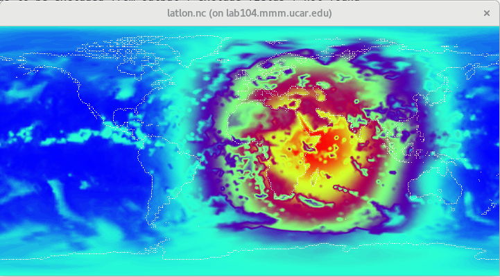
Now that we have the top-of-the-atmosphere accumulated net radiative energy flux integrated over two six-hour periods from our
12-hour simulation, we can compute a radiation budget (in W / m^2) for these time periods with a Python script.
Using an editor of your choice, create a file named compute_budget.py with the following contents:
import numpy as np
from netCDF4 import Dataset

f = Dataset('accradflux.2014-09-10_12.00.00.nc')
accradflux = f.variables['accradflux'][:]

g = Dataset('x1.10242.init.nc')
areaCell = g.variables['areaCell'][:]

print(np.sum(accradflux * areaCell) / np.sum(areaCell) / 21600.0)
We can run this script with:
$ python compute_budget.py
You can try changing the time perdiod for which this radiation budget is computed by changing 'accradflux.2014-09-10_12.00.00.nc'
to 'accradflux.2014-09-10_06.00.00.nc' in the script.
Positive values indicate more incoming radiation at the top of the atmosphere than outgoing radiation.
With the remaining time in this session, you may like to try one of the following:
- Run a multi-day simulation, writing the "toa_energy_balance" stream only once per day; then, compute the radiation budget
for 24-hour periods using a modified version of the Python script described above
- Run a two-day simulation, writing the "toa_energy_balance" stream every three hours; then, compute the radiation budget
for these three-hour periods and note how the resulting values change during the simulation.
IMPORTANT NOTE:By default the MPAS stream manager will refuse
to overwrite any existing output files. Before re-running simulations, you will generally
need to remove previous model output files with:
$ rm diag*nc history*nc surface_winds*nc accradflux*nc restart*nc
However, as described in Section 5.2 of the MPAS-Atmosphere User's Guide, you can set the
clobber_mode attribute for output streams so that any existing
files will be overwritten.
As an example of processing multiple NetCDF files in a loop in Python, you can use the following script:
import numpy as np
from netCDF4 import Dataset

g = Dataset('x1.10242.init.nc')
areaCell = g.variables['areaCell'][:]
g.close()

for filename in ['accradflux.2014-09-10_00.00.00.nc',
                 'accradflux.2014-09-11_00.00.00.nc',
                 'accradflux.2014-09-12_00.00.00.nc']:

        f = Dataset(filename)
        accradflux = f.variables['accradflux'][:]
        f.close()

        print(np.sum(accradflux * areaCell) / np.sum(areaCell) / 86400.0)