Inertia-Gravity Waves

The test cases for inertia-gravity (IG) waves are described in Skamarock and Klemp, 1994: Efficiency and Accuracy of the Klemnp-Wilhelmson Time-Splitting Technique, Mon. Wea. Rev.,  122, 2623-2630.  There are two tests described in the paper - tests for hydrostatic and nonhydrostatic-scale waves.

Both test cases use a mean wind to translate the evolving IG waves - this provides an indication of phase errors associated with gravity waves propagating both with and against the mean flow; the solutions should be symmetric about the center of the translating initial perturbation. 

The hydrostatic test case is a good test for determining if the maximum allowable timesteps in a nonhydrostatic model configured for hydrostatic resolutions is consistent with expectations given the model formulation.   Implicit or time-split explicit treatment of the gravity waves will be needed if large timesteps are to be stable (as in hydrostatic models).

The nonhydrostatic test case provides a test of timestep size and solution accuracy for a grid of aspect-ratio (dz/dx) = 1. 

The results in the paper and shown below are for a model using the Boussinesq approximation.  Also shown are results for the WRF-ARW model which integrates the fully compressible equations.   The solutions exhibit some qualitative differences,  but the tests can be revealing for both model types.  Also included are solutions from the ARPS model which uses leapfrog time integration and a 2nd order advection scheme.

13 October 2005, W. Skamarock
12 December 2005, added Coriolis parameter value, note on ARW contour intervals, W. Skamarock

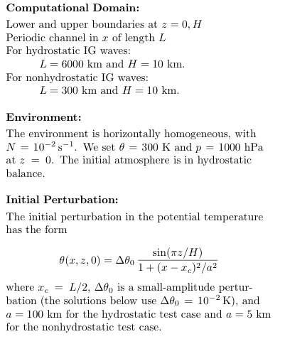
Note: for the hydrostatic test case, the Coriolis parameter f = 10**(-4)/s (this information is missing from the paper).

Solutions from the Boussinesq model (from Skamarock and Klemp 1994)

________________________________________________________

Mean wind U = 20 m/s, 3000 second result for the nonhydrostatic IG waves.

________________________________________________________

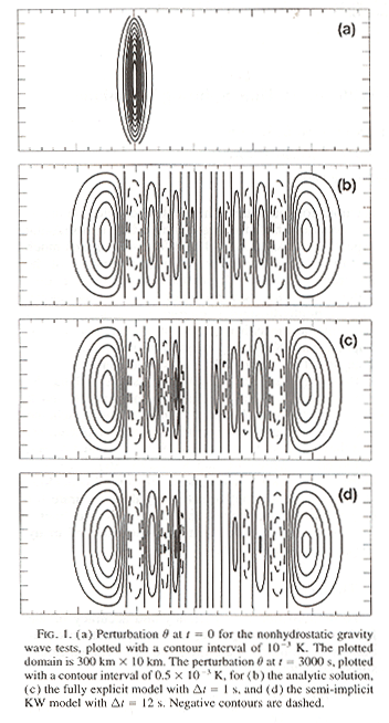
Mean wind U = 20 m/s, 60,000 second result for the hydrostatic IG waves.

________________________________________________________

________________________________________________________
 
Solutions from the WRF-ARW model (http://wrf-model.org) and the ARPS model (http://www.caps.ou.edu/ARPS; from the Users' Guide).  Reference solutions (using no mean horizontal wind and twice the resolution as used in Skamarock and Klemp 1994) are included. 

Note: The perturbation used in the WRF-ARW model has an amplitude of 0.1 K as opposed to 0.01 K used in the Skamarock and Klemp (1994) paper (the ARW model was run in single precision and as such is more sensitive to machine roundoff error), so the contour interval is an order of magnitude higher in the ARW plots below.  The ARPS solutions use a 0.01 K perturbation (and the same contour interval) as in Skamarock and Klemp (1994).

________________________________________________________

Nonhydrostatic-scale solutions

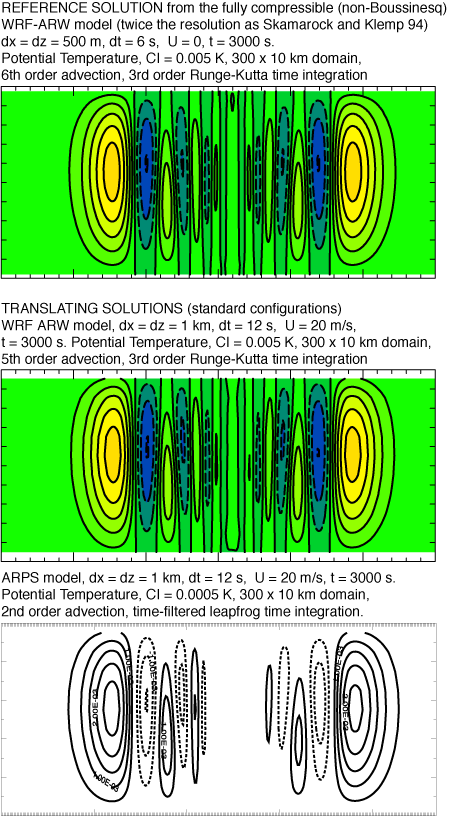
From the ARPS Version 4.0 Users Guide, Fig 13.6.  In comparing the WRF-ARW and ARPS solutions, it should be noted that the WRF-ARW model uses a constant pressure upper boundary condition (ARW has a hydrostatic pressure vertical coordinate)  whereas ARPS uses a rigid lid upper boundary (ARPS has a geometric height vertical coordinate).  This leads to small differences in the solutions.  More noticable in the comparison are the larger phase errors associated with the ARPS solutions, as expected given the lower order temporal and spatial integration schemes used in ARPS compared with WRF-ARW.

________________________________________________________

Hydrostatic-scale solutions

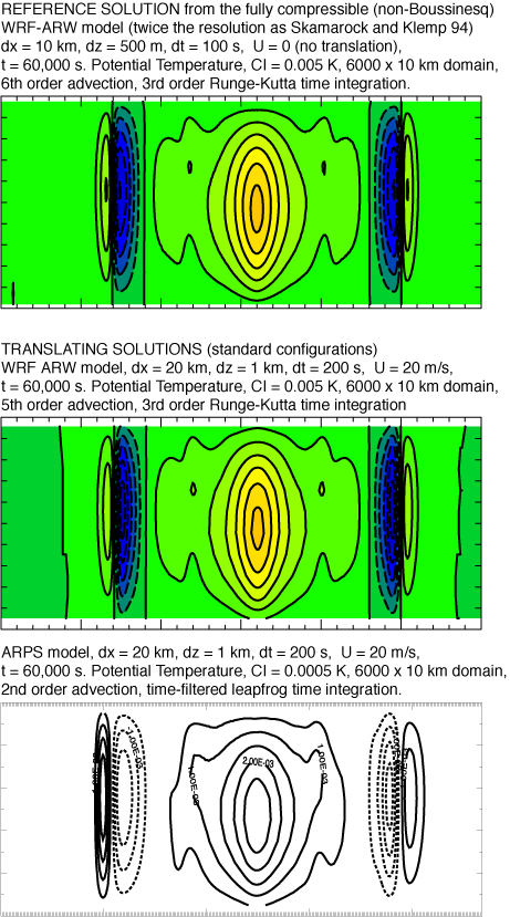
From the ARPS Version 4.0 Users Guide, Fig 13.7.  In comparing the WRF-ARW and ARPS solutions, it should be noted that the WRF-ARW model uses a constant pressure upper boundary condition (ARW has a hydrostatic pressure vertical coordinate)  whereas ARPS uses a rigid lid upper boundary (ARPS has a geometric height vertical coordinate).  This leads to small differences in the solutions.  More noticable in the comparison are the larger phase errors associated with the ARPS solutions, as expected given the lower order temporal and spatial integration schemes used in ARPS compared with WRF-ARW.