For climate runs, reanalysis or future climate model data are the best sources of data, as it provides a continuous data source.

SST is very important in climate runs, so we need a good source of SST, and we need to ensure the SST is updated throughout climate simulations.

As this is a test case, we are only running for 48 hours. Typically, these runs will be months or years.

1. Run the Geogrid Program

1. At this time, you may want to consider creating a new folder in which to save your met_em* files from previous runs, along with your namelist.wps file, in case you want to use them later, and do not want to re-run everything from scratch.  


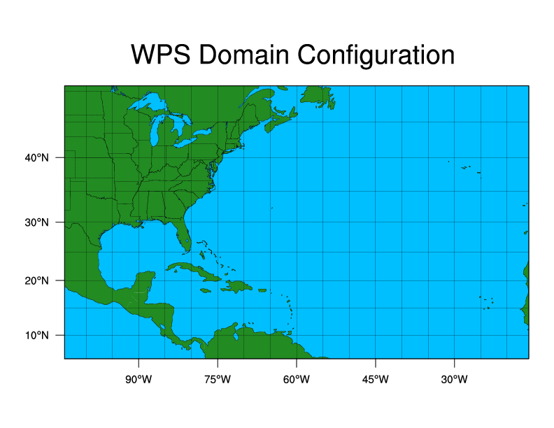
2. We are going to create a single domain over North America and the North Atlantic. Edit namelist.wps to reflect the following parameterizations:
   
   
   • The domain size will be 110x65 grid points.
   
   
   • The grid resolution will be 90km.
     
     

     Note:
     Downscaled climate simulations will typically be at a higher resolution than 90km, but since this is just a test case, and we would like to cover a large area, we compromised on the resolution).

   
   
   • We will use a Mercator projection.
   
   
   • To place the domain in the right location on the Earth, make the following additional changes to the namelist:

     &geogrid
     max_dom = 1,
     ref_lat = 30.00
     ref_lon = -60.00
     truelat1 = 0.0,
     truelat2 = 0.0,
     stand_lon = -60.00
     



3. The above domain should look like this:
   

   

    

4. Run geogrid

2. Run the Ungrib Program

Degrib and reformat meteorological data from reanalysis or climate models. In this case, the data come from NCEP CFSv2 Climate Forecast System, and archived SST. We are going to ungrib the two datasets separately.

1. First link the CFSv2 data using the script file link_grib.csh:
    
   ./link_grib.csh    /home/ec2-user/input_data/CFSV2/cdas1.2016100   
    
   
2. Link the correct Vtable (the input data for this case is CFS, so use the CFSR Vtable).



3. Case dates are 2016-10-06_00 to 2016-10-08_00, and data are available 6-hourly.
   Make the appropriate changes to the namelist to correctly ingest the data for the right times and interval.
   
    
4. Run ungrib to create the intermediate files (these files should have the prefix "FILE").



5. Second, link the SST data using the script file link_grib.csh:
    
   ./link_grib.csh    /home/ec2-user/input_data/SST/rtg_sst_grb_hr_0.083.2016100   
   
    
   
6. Link the correct Vtable (the input data for this case is SST, so use the SST Vtable)
   
   
7. Make the following changes to &ungrib section of the namelist to correctly ingest the data for the right times.

   &ungrib
   prefix = 'SST',

   Notes:

   • The interval between the SST data sets is 24 hours. We need SST data 6-hourly to match the NCEP2 data interval. By keeping 'interval_seconds' set to 21600, we can interpolate our available data to the required 6-hourly intervals.
   
   
   • Note the prefix change - this is so that we do not overwrite the CFSv2 data we just ungribbed.
   
   
   • If our SST data had been only been available, say weekly, we would have changed the namelist date range to the 2 available dates, before and after our case dates, and we would keep 'interval_seconds = 21600' to interpolate.
 
8. Run ungrib to create intermediate files for SST data (the prefix of these files will be "SST").

3. Run the Metgrid Program

1. Before running metgrid.exe, first make the following change to the &metgrid section of the namelist to ensure both FILE and SST files created by ungrib will be used by metgrid:

   &metgrid
   fg_name = 'FILE', 'SST'




2. Now - run metgrid, as usual. (Note: You will get warning messages regarding the variable DEWPT. This only indicates that the variable DEWPT was found in the data, but is not found in the METGRID.TBL, which is okay because we will use specific humidity in the WRF model. You can ignore this warning message and continue).
   

4. Set-up and Run WRF

 
1. Edit the namelist.input file to match the settings you used for WPS.

   Notes:

   • Set "frames_per_outfile" to 1 - this will create a new wrfout file for each output time - this is a good option for long runs, as it makes the output more manageable.
   
   
   • For long runs, you will likely need to stop and start often, so create restart files at least once a day.
   
   
   • Pay attention to the time step. Since we are running on a 90km domain, this can be larger. Typically the rule is 6xDX, but to ensure stability, set this to 360.
   
   
   • Be careful to not use too few vertical levels when doing long simulations, as this could lead to systematic biases. 35 levels should be okay for this case.
   
   
   • Set "p_top_requested" to 50 hPa. Note that we can only do so if our input data include this level (which ours does). Secondly, long simulations benefit from a higher model top, so always try to obtain data with a top of at least 10mb.
      
   
   
   
   
2. Now add the following to the namelist.input file under the &time_control and &physics sections

   &time_control
   auxinput4_inname = "wrflowinp_d<domain>"
   auxinput4_interval = 360,
   io_form_auxinput4 = 2,
    
   &physics
   sst_update = 1,

   Notes:

   • The addition of these lines will ensure the model updates SST every 6 hours throughout the simulation. SST uses the auxillary stream 4, so we have to specify the file name that will be created when real.exe is run, the interval, and what type of output we want these files to be (2=netcdf).
   
   
   • Do not change the syntax for the auxinput4_inname parameter. WRF understand this syntax and will correctly translate that to the correct file name.  
   
   
   
3. Now you are ready to run real and wrf.

 
 

If this was successful, you can continue to another exercise.