Chapter 9: Post-Processing Utilities

Table of Contents

· Introduction

· NCL

· RIP4

· ARWpost

· UPP

· VAPOR

Introduction

There are a number of visualization tools available to display WRF-ARW (http:// http://www2.mmm.ucar.edu/wrf/users) model data. Model data in netCDF format can essentially be displayed using any tool capable of displaying this data format.

Currently the following post-processing utilities are supported: NCL, RIP4, ARWpost (converter to GrADS), UPP, and VAPOR.

NCL, RIP4, ARWpost and VAPOR can currently only read data in netCDF format, while UPP can read data in netCDF and binary format.

Required software

The only library that is always required is the netCDF package from Unidata (http://www.unidata.ucar.edu/: login > Downloads > NetCDF - registration login required).

netCDF stands for Network Common Data Form. This format is platform independent, i.e., data files can be read on both big-endian and little-endian computers, regardless of where the file was created. To use the netCDF libraries, ensure that the paths to these libraries are set correct in your login scripts as well as all Makefiles.

Additional libraries required by each of the supported post-processing packages:

· NCL (http://www.ncl.ucar.edu)

· GrADS (http://grads.iges.org/home.html)

· GEMPAK (http://www.unidata.ucar.edu/software/gempak/)

· VAPOR (http://www.vapor.ucar.edu)

NCL

With the use of NCL Libraries (http://www.ncl.ucar.edu), WRF-ARW data can easily be displayed.

The information on these pages has been put together to help users generate NCL scripts to display their WRF-ARW model data.

Some example scripts are available online

(http://www2.mmm.ucar.edu/wrf/OnLineTutorial/Graphics/NCL/NCL_examples.htm), but in order to fully utilize the functionality of the NCL Libraries, users should adapt these for their own needs, or write their own scripts.

NCL can process WRF-ARW static, input and output files, as well as WRFDA output data. Both single and double precision data can be processed.

WRF and NCL

In July 2007, the WRF-NCL processing scripts have been incorporated into the NCL Libraries, thus only the NCL Libraries are now needed.

Major WRF-ARW-related upgrades have been added to the NCL libraries in version 6.1.0; therefore, in order to use many of the functions, NCL version 6.1.0 or higher is required.

Special functions are provided to simplify the plotting of WRF-ARW data. These functions are located in:

"$NCARG_ROOT/lib/ncarg/nclscripts/wrf/WRFUserARW.ncl".
Users are encouraged to view and edit this file for their own needs. If users wish to edit this file, but do not have write permission, they should simply copy the file to a local directory, edit and load the new version, when running NCL scripts.

Special NCL built-in functions have been added to the NCL libraries to help users calculate basic diagnostics for WRF-ARW data. 

All the FORTRAN subroutines used for diagnostics and interpolation (previously located in wrf_user_fortran_util_0.f) has been re-coded into NCL in-line functions. This means users no longer need to compile these routines.

What is NCL

The NCAR Command Language (NCL) is a free, interpreted language designed specifically for scientific data processing and visualization. NCL has robust file input and output. It can read in netCDF, HDF4, HDF4-EOS, GRIB, binary and ASCII data. The graphics are world-class and highly customizable.

It runs on many different operating systems including Solaris, AIX, IRIX, Linux, MacOSX, Dec Alpha, and Cygwin/X running on Windows. The NCL binaries are freely available at: http://www.ncl.ucar.edu/Download/

To read more about NCL, visit: http://www.ncl.ucar.edu/overview.shtml

Necessary software

NCL libraries, version 6.1.0 or higher.

Environment Variable

Set the environment variable NCARG_ROOT to the location where you installed the NCL libraries. Typically (for cshrc shell):

setenv NCARG_ROOT /usr/local/ncl

.hluresfile

Create a file called .hluresfile in your $HOME directory. This file controls the color, background, fonts, and basic size of your plot. For more information regarding this file, see: http://www.ncl.ucar.edu/Document/Graphics/hlures.shtml.

NOTE: This file must reside in your $HOME directory and not where you plan on running NCL.

Below is the .hluresfile used in the example scripts posted on the web (scripts are available at: http://www2.mmm.ucar.edu/wrf/users/graphics/NCL/NCL.htm). If a different color table is used, the plots will appear different. Copy the following to your ~/.hluresfile. (A copy of this file is available at:

http://www2.mmm.ucar.edu/wrf/OnLineTutorial/Graphics/NCL/NCL_basics.htm)

*wkColorMap : BlAqGrYeOrReVi200

*wkBackgroundColor : white

*wkForegroundColor : black

*FuncCode : ~

*TextFuncCode : ~

*Font : helvetica

*wkWidth : 900

*wkHeight : 900

NOTE:

If your image has a black background with white lettering, your .hluresfile has not been created correctly, or it is in the wrong location.

wkColorMap, as set in your .hluresfile can be overwritten in any NCL script with the use of the function “gsn_define_colormap”, so you do not need to change your .hluresfile if you just want to change the color map for a single plot.

Create NCL scripts

The basic outline of any NCL script will look as follows:

load external functions and procedures

begin

; Open input file(s)

; Open graphical output

; Read variables

; Set up plot resources & Create plots

; Output graphics

end

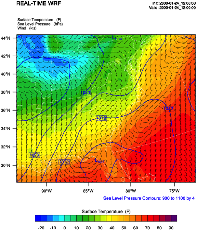
For example, let’s create a script to plot Surface Temperature, Sea Level Pressure and Wind as shown in the picture below.

; load functions and procedures

load "$NCARG_ROOT/lib/ncarg/nclscripts/csm/gsn_code.ncl"

load "$NCARG_ROOT/lib/ncarg/nclscripts/wrf/WRFUserARW.ncl"

begin

; WRF ARW input file (NOTE, your wrfout file does not need
; the .nc, but NCL needs it so make sure to add it in the
; line below)
a = addfile("../wrfout_d01_2000-01-24_12:00:00.nc","r")

; Output on screen. Output will be called "plt_Surface1"

type = "x11"

wks = gsn_open_wks(type,"plt_Surface1")

; Set basic resources

res = True

res@MainTitle = "REAL-TIME WRF" ; Give plot a main title

res@Footer = False ; Set Footers off
pltres = True ; Plotting resources
mpres = True ; Map resources

;---------------------------------------------------------------

times = wrf_user_getvar(a,"times",-1)) ; get times in the file

it = 0 ; only interested in first time

res@TimeLabel = times(it) ; keep some time information

;---------------------------------------------------------------

; Get variables

slp = wrf_user_getvar(a,"slp",it) Get slp

wrf_smooth_2d( slp, 3 ) ; Smooth slp

t2 = wrf_user_getvar(a,"T2",it) ; Get T2 (deg K)

   tc2 = t2-273.16 ; Convert to deg C

   tf2 = 1.8*tc2+32. ; Convert to deg F

   tf2@description = "Surface Temperature"

   tf2@units = "F"

u10 = wrf_user_getvar(a,"U10",it) ; Get U10

v10 = wrf_user_getvar(a,"V10",it) ; Get V10

   u10 = u10*1.94386 ; Convert to knots

   v10 = v10*1.94386

   u10@units = "kts"

   v10@units = "kts"

;---------------------------------------------------------------

; Plotting options for T

opts = res ; Add basic resources

opts@cnFillOn = True ; Shaded plot

opts@ContourParameters = (/ -20., 90., 5./) ; Contour intervals

opts@gsnSpreadColorEnd = -3

contour_tc = wrf_contour(a,wks,tf2,opts) ; Create plot

delete(opts)

; Plotting options for SLP

opts = res ; Add basic resources

opts@cnLineColor = "Blue" ; Set line color

opts@cnHighLabelsOn = True ; Set labels

opts@cnLowLabelsOn = True

opts@ContourParameters = (/ 900.,1100.,4./) ; Contour intervals

contour_psl = wrf_contour(a,wks,slp,opts) ; Create plot delete(opts)

; Plotting options for Wind Vectors

opts = res ; Add basic resources

opts@FieldTitle = "Winds" ; Overwrite the field title

opts@NumVectors = 47 ; Density of wind barbs

vector = wrf_vector(a,wks,u10,v10,opts) ; Create plot

delete(opts)

; MAKE PLOTS 

plot = wrf_map_overlays(a,wks, \
(/contour_tc,contour_psl,vector/),pltres,mpres)

;---------------------------------------------------------------

end

Extra sample scripts are available at: http://www2.mmm.ucar.edu/wrf/OnLineTutorial/Graphics/NCL/NCL_examples.htm

Run NCL scripts

1. Ensure NCL is successfully installed on your computer.

2. Ensure that the environment variable NCARG_ROOT is set to the location where NCL is installed on your computer. Typically (for cshrc shell), the command will look as follows:

setenv NCARG_ROOT /usr/local/ncl

3. Create an NCL plotting script.

4. Run the NCL script you created:

ncl NCL_script

The output type created with this command is controlled by the line:

wks = gsn_open_wk (type,"Output") ; inside the NCL script
where type can be x11, pdf, ncgm, ps, or eps

For high quality images, create pdf , ps, or eps images directly via the ncl scripts (type = pdf / ps / eps)

See the Tools section in Chapter 10 of this User’s Guide for more information concerning other types of graphical formats and conversions between graphical formats.

Functions / Procedures under "$NCARG_ROOT/lib/ncarg/nclscripts/wrf/" (WRFUserARW.ncl)

wrf_user_getvar (nc_file, fld, it)

Usage: ter = wrf_user_getvar (a, “HGT”, 0)

Get fields from a netCDF file for:

· Any given time by setting it to the time required.

· For all times in the input file(s), by setting it = -1

· A list of times from the input file(s), by setting it to (/start_time,end_time,interval/) ( e.g. (/0,10,2/) ).

· A list of times from the input file(s), by setting it to the list required ( e.g. (/1,3,7,10/) ).

Any field available in the netCDF file can be extracted.

fld is case sensitive. The policy adapted during development was to set all diagnostic variables, calculated by NCL, to lower-case to distinguish them from fields directly available from the netCDF files.

List of available diagnostics:

avo	Absolute Vorticity [10-5 s-1]
pvo	Potential Vorticity [PVU]
eth	Equivalent PotentialTtemperature [K]
cape_2d	Returns 2D fields mcape/mcin/lcl/lfc
cape_3d	Returns 3D fields cape/cin
dbz	Reflectivity [dBZ]
mdbz	Maximum Reflectivity [dBZ]
geopt/geopotential	Full Model Geopotential [m2 s-2]
helicity	Storm Relative Helicity [m-2/s-2]
updraft_helicity	Updraft Helicity [m-2/s-2]
lat	Latitude (will return either XLAT or XLAT_M, depending on which is available)
lon	Longitude (will return either XLONG or XLONG_M, depending on which is available)
omg	Omega
p/pres	Full Model Pressure [Pa]
pressure	Full Model Pressure [hPa]
pw	Precipitable Water
rh2	2m Relative Humidity [%]
rh	Relative Humidity [%]
slp	Sea Level Pressure [hPa]
ter	Model Terrain Height [m] (will return either HGT or HGT_M, depending on which is available)
td2	2m Dew Point Temperature [C]
td	Dew Point Temperature [C]
tc	Temperature [C]
tk	Temperature [K]
th/theta	Potential Temperature [K]
tv	Virtual Temperature
twb	Wetbulb Temperature
times	Times in file (note this return strings - recommended)
Times	Times in file (note this return characters)
ua	U component of wind on mass points
va	V component of wind on mass points
wa	W component of wind on mass points
uvmet10	10m U and V components of wind rotated to earth coordinates
uvmet	U and V components of wind rotated to earth coordinates
z/height	Full Model Height [m]

wrf_user_list_times (nc_file)

Usage: times = wrf_user_list_times (a)

Obtain a list of times available in the input file. The function returns a 1D array containing the times (type: character) in the input file.

This is an outdated function – best to use wrf_user_getvar(nc_file,”times”,it)

wrf_contour (nc_file, wks, data, res)

Usage: contour = wrf_contour (a, wks, ter, opts)

Returns a graphic (contour), of the data to be contoured. This graphic is only created, but not plotted to a wks. This enables a user to generate many such graphics and overlay them, before plotting the resulting picture to the wks.

The returned graphic (contour) does not contain map information, and can therefore be used for both real and idealized data cases.

This function can plot both line contours and shaded contours. Default is line contours.

Many resources are set for a user, and most can be overwritten. Below is a list of resources you may want to consider changing before generating your own graphics:

Resources unique to ARW WRF Model data

opts@MainTitle : Controls main title on the plot.

opts@MainTitlePos : Main title position – Left/Right/Center. Default is Left.

opts@NoHeaderFooter : Switch off all Headers and Footers.

opts@Footer : Add some model information to the plot as a footer. Default is True.

opts@InitTime : Plot initial time on graphic. Default is True. If True, the initial time will be extracted from the input file.

opts@ValidTime : Plot valid time on graphic. Default is True. A user must set opts@TimeLabel to the correct time.

opts@TimeLabel : Time to plot as valid time.

opts@TimePos : Time position – Left/Right. Default is “Right”.

opts@ContourParameters : A single value is treated as an interval. Three values represent: Start, End, and Interval.

opts@FieldTitle : Overwrite the field title - if not set the field description is used for the title.

opts@UnitLabel : Overwrite the field units - seldom needed as the units associated with the field will be used.

opts@PlotLevelID : Use to add level information to the field title.

General NCL resources (most standard NCL options for cn and lb can be set by the user to overwrite the default values)

opts@cnFillOn : Set to True for shaded plots. Default is False.

opts@cnLineColor : Color of line plot.

opts@lbTitleOn : Set to False to switch the title on the label bar off. Default is True.

opts@cnLevelSelectionMode ; opts @cnLevels ; opts@cnFillColors ; optr@cnConstFLabelOn : Can be used to set contour levels and colors manually. 

wrf_vector (nc_file, wks, data_u, data_v, res)

Usage: vector = wrf_vector (a, wks, ua, va, opts)

Returns a graphic (vector) of the data. This graphic is only created, but not plotted to a wks. This enables a user to generate many graphics, and overlay them, before plotting the resulting picture to the wks.

The returned graphic (vector) does not contain map information, and can therefore be used for both real and idealized data cases.

Many resources are set for a user, and most can be overwritten. Below is a list of resources you may want to consider changing before generating your own graphics:

Resources unique to ARW WRF Model data

opts@MainTitle : Controls main title on the plot.

opts@MainTitlePos : Main title position – Left/Right/Center. Default is Left.

opts@NoHeaderFooter : Switch off all Headers and Footers.

opts@Footer : Add some model information to the plot as a footer. Default is True.

opts@InitTime : Plot initial time on graphic. Default is True. If True, the initial time will be extracted from the input file.

opts@ValidTime : Plot valid time on graphic. Default is True. A user must set opts@TimeLabel to the correct time.

opts@TimeLabel : Time to plot as valid time.

opts@TimePos : Time position – Left/Right. Default is “Right”.

opts@ContourParameters : A single value is treated as an interval. Three values represent: Start, End, and Interval.

opts@FieldTitle : Overwrite the field title - if not set the field description is used for the title.

opts@UnitLabel : Overwrite the field units - seldom needed as the units associated with the field will be used.

opts@PlotLevelID : Use to add level information to the field title.

opts@NumVectors : Density of wind vectors.

General NCL resources (most standard NCL options for vc can be set by the user to overwrite the default values)

opts@vcGlyphStyle : Wind style. “WindBarb” is default. 

wrf_map_overlays (nc_file, wks, (/graphics/), pltres, mpres)

Usage: plot = wrf_map_overlays (a, wks, (/contour,vector/), pltres, mpres)

Overlay contour and vector plots generated with wrf_contour and wrf_vector. Can overlay any number of graphics. Overlays will be done in the order given, so always list shaded plots before line or vector plots, to ensure the lines and vectors are visible and not hidden behind the shaded plot.

A map background will automatically be added to the plot. Map details are controlled with the mpres resource. Common map resources you may want to set are:

mpres@mpGeophysicalLineColor ; mpres@mpNationalLineColor ; mpres@mpUSStateLineColor ; mpres@mpGridLineColor ; mpres@mpLimbLineColor ; mpres@mpPerimLineColor

If you want to zoom into the plot, set mpres@ZoomIn to True, and mpres@Xstart, mpres@Xend, mpres@Ystart, and mpres@Yend to the corner x/y positions of the zoomed plot.

pltres@NoTitles : Set to True to remove all field titles on a plot.

pltres@CommonTitle : Overwrite field titles with a common title for the overlaid plots. Must set pltres@PlotTitle to desired new plot title.

If you want to generate images for a panel plot, set pltres@PanelPot to True.

If you want to add text/lines to the plot before advancing the frame, set pltres@FramePlot to False. Add your text/lines directly after the call to the wrf_map_overlays function. Once you are done adding text/lines, advance the frame with the command “frame (wks)”.

wrf_overlays (nc_file, wks, (/graphics/), pltres)

Usage: plot = wrf_overlays (a, wks, (/contour,vector/), pltres)

Overlay contour and vector plots generated with wrf_contour and wrf_vector. Can overlay any number of graphics. Overlays will be done in the order given, so always list shaded plots before line or vector plots, to ensure the lines and vectors are visible and not hidden behind the shaded plot.

Typically used for idealized data or cross-sections, which does not have map background information.

pltres@NoTitles : Set to True to remove all field titles on a plot.

pltres@CommonTitle : Overwrite field titles with a common title for the overlaid plots. Must set pltres@PlotTitle to desired new plot title.

If you want to generate images for a panel plot, set pltres@PanelPot to True.

If you want to add text/lines to the plot before advancing the frame, set pltres@FramePlot to False. Add your text/lines directly after the call to the wrf_overlays function. Once you are done adding text/lines, advance the frame with the command “frame (wks)”.

wrf_map (nc_file, wks, res)

Usage: map = wrf_map (a, wks, opts)

Create a map background.

As maps are added to plots automatically via the wrf_map_overlays function, this function is seldom needed as a stand-alone.

wrf_user_intrp3d (var3d, H, plot_type, loc_param, angle, res)

This function is used for both horizontal and vertical interpolation.

var3d: The variable to interpolate. This can be an array of up to 5 dimensions. The 3 right-most dimensions must be bottom_top x south_north x west_east.

H: The field to interpolate to. Either pressure (hPa or Pa), or z (m). Dimensionality must match var3d.

plot_type: “h” for horizontally- and “v” for vertically-interpolated plots.

loc_param: Can be a scalar, or an array, holding either 2 or 4 values.

For plot_type = “h”:

This is a scalar representing the level to interpolate to.

Must match the field to interpolate to (H).

When interpolating to pressure, this can be in hPa or Pa (e.g. 500., to interpolate to 500 hPa). When interpolating to height this must in in m (e.g. 2000., to interpolate to 2 km).

For plot_type = “v”:

This can be a pivot point though which a line is drawn – in this case a single x/y point (2 values) is required. Or this can be a set of x/y points (4 values), indicating start x/y and end x/y locations for the cross-section.

angle:

Set to 0., for plot_type = “h”, or for plot_type = “v” when start and end locations of cross-section are supplied in loc_param.

If a single pivot point was supplied in loc_param, angle is the angle of the line that will pass through the pivot point. Where: 0. is SN, and 90. is WE.

res:

Set to False for plot_type = “h”, or for plot_type = “v” when a single pivot point is supplied. Set to True if start and end locations are supplied. 

wrf_user_intrp2d (var2d, loc_param, angle, res)

This function interpolates a 2D field along a given line.

var2d: The 2D field to interpolate. This can be an array of up to 3 dimensions. The 2 right-most dimensions must be south_north x west_east.

loc_param:

An array holding either 2 or 4 values.

This can be a pivot point though which a line is drawn - in this case a single x/y point (2 values) is required. Or this can be a set of x/y points (4 values), indicating start x/y and end x/y locations for the cross-section.

angle:

Set to 0 when start and end locations of the line are supplied in loc_param.

If a single pivot point is supplied in loc_param, angle is the angle of the line that will pass through the pivot point. Where: 0. is SN, and 90. is WE.

res:

Set to False when a single pivot point is supplied. Set to True if start and end locations are supplied. 

wrf_user_ll_to_ij (nc_file, lons, lats, res)

Usage: loc = wrf_user_latlon_to_ij (a, 100., 40., res)

Usage: loc = wrf_user_latlon_to_ij (a, (/100., 120./), (/40., 50./), res)

Converts a lon/lat location to the nearest x/y location. This function makes use of map information to find the closest point; therefore this returned value may potentially be outside the model domain.

lons/lats can be scalars or arrays.

Optional resources:

res@returnInt - If set to False, the return values will be real (default is True with integer return values)

res@useTime - Default is 0. Set if you want the reference longitude/latitudes to come from a specific time - one will only use this for moving nest output, which has been stored in a single file.

loc(0,:) is the x (WE) locations, and loc(1,:) the y (SN) locations.

wrf_user_ij_to_ll (nc_file, i, j, res)

Usage: loc = wrf_user_latlon_to_ij (a, 10, 40, res)

Usage: loc = wrf_user_latlon_to_ij (a, (/10, 12/), (/40, 50/), res)

Convert an i/j location to a lon/lat location. This function makes use of map information to find the closest point, so this returned value may potentially be outside the model domain.

i/j can be scalars or arrays.

Optional resources:

res@useTime - Default is 0. Set if you want the reference longitude/latitudes to come from a specific time - one will only use this for moving nest output, which has been stored in a single file.

loc(0,:) is the lons locations, and loc(1,:) the lats locations.

wrf_user_unstagger (varin, unstagDim)

This function unstaggers an array, and returns an array on ARW WRF mass points.

varin: Array to be unstaggered.

unstagDim: Dimension to unstagger. Must be either "X", "Y", or "Z". This is case sensitive. If you do not use one of these strings, the returning array will be unchanged.

wrf_wps_dom (wks, mpres, lnres, txres)

A function has been built into NCL to preview where a potential domain will be placed (similar to plotgrids.exe from WPS).

The lnres and txres resources are standard NCL Line and Text resources. These are used to add nests to the preview.

The mpres are used for standard map background resources like:

mpres@mpFillOn ; mpres@mpFillColors ; mpres@mpGeophysicalLineColor ; mpres@mpNationalLineColor ; mpres@mpUSStateLineColor ; mpres@mpGridLineColor ; mpres@mpLimbLineColor ; mpres@mpPerimLineColor

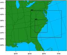
Its main function, however, is to set map resources to preview a domain. These resources are similar to the resources set in WPS. Below is an example of how to display 3 nested domains on a Lambert projection. (The output is shown below).

mpres@max_dom = 3

mpres@parent_id = (/ 1, 1, 2 /)

mpres@parent_grid_ratio = (/ 1, 3, 3 /)

mpres@i_parent_start = (/ 1, 31, 15 /)

mpres@j_parent_start = (/ 1, 17, 20 /)

mpres@e_we = (/ 74, 112, 133/)

mpres@e_sn = (/ 61, 97, 133 /)

mpres@dx = 30000.

mpres@dy = 30000.

mpres@map_proj = "lambert"

mpres@ref_lat = 34.83

mpres@ref_lon = -81.03

mpres@truelat1 = 30.0

mpres@truelat2 = 60.0

mpres@stand_lon = -98.0

NCL built-in Functions

A number of NCL built-in functions have been created to help users calculate simple diagnostics. Full descriptions of these functions are available on the NCL web site (http://www.ncl.ucar.edu/Document/Functions/wrf.shtml).

wrf_avo	Calculates absolute vorticity.
wrf_cape_2d	Computes convective available potential energy (CAPE), convective inhibition (CIN), lifted condensation level (LCL), and level of free convection (LFC).
wrf_cape_3d	Computes convective available potential energy (CAPE) and convective inhibition (CIN).
wrf_dbz	Calculates the equivalent reflectivity factor.
wrf_eth	Calculates equivalent potential temperature
wrf_helicity	Calculates storm relative helicity
wrf_ij_to_ll	Finds the longitude, latitude locations to the specified model grid indices (i,j).
wrf_ll_to_ij	Finds the model grid indices (i,j) to the specified location(s) in longitude and latitude.
wrf_omega	Calculates omega
wrf_pvo	Calculates potential vorticity.
wrf_rh	Calculates relative humidity.
wrf_slp	Calculates sea level pressure.
wrf_smooth_2d	Smooth a given field.
wrf_td	Calculates dewpoint temperature in [C].
wrf_tk	Calculates temperature in [K].
wrf_updraft_helicity	Calculates updraft helicity
wrf_uvmet	Rotates u,v components of the wind to earth coordinates.
wrf_virual_temp	Calculates virtual temperature
wrf_wetbulb	Calculates wetbulb temperature

Adding diagnostics using FORTRAN code

It is possible to link your favorite FORTRAN diagnostics routines to NCL. It is easier to use FORTRAN 77 code, but NCL also recognizes basic FORTRAN 90 code.

Let’s use a routine that calculates temperature (K) from theta and pressure.

FORTRAN 90 routine called myTK.f90

subroutine compute_tk (tk, pressure, theta, nx, ny, nz)
implicit none

!! Variables

integer :: nx, ny, nz

real, dimension (nx,ny,nz) :: tk, pressure, theta

!! Local Variables

integer :: i, j, k
real, dimension (nx,ny,nz):: pi

pi(:,:,:) = (pressure(:,:,:) / 1000.)**(287./1004.)
tk(:,:,:) = pi(:,:,:)*theta(:,:,:)

return
end subroutine compute_tk

For simple routines like this, it is easiest to re-write the routine into a FORTRAN 77 routine.

FORTRAN 77 routine called myTK.f

subroutine compute_tk (tk, pressure, theta, nx, ny, nz)
implicit none

C Variables

integer nx, ny, nz

real tk(nx,ny,nz) , pressure(nx,ny,nz), theta(nx,ny,nz)

C Local Variables

integer i, j, k
real pi

DO k=1,nz
DO j=1,ny
DO i=1,nx
pi=(pressure(i,j,k) / 1000.)**(287./1004.)
tk(i,j,k) = pi*theta(i,j,k)
ENDDO
ENDDO

ENDDO

return
end

Add the markers NCLFORTSTART and NCLEND to the subroutine as indicated below. Note, that local variables are outside these block markers.

FORTRAN 77 routine called myTK.f, with NCL markers added

C NCLFORTSTART

subroutine compute_tk (tk, pressure, theta, nx, ny, nz)
implicit none

C Variables

integer nx, ny, nz

real tk(nx,ny,nz) , pressure(nx,ny,nz), theta(nx,ny,nz)

C NCLEND

C Local Variables

integer i, j, k
real pi

DO k=1,nz
DO j=1,ny
DO i=1,nx
pi=(pressure(i,j,k) / 1000.)**(287./1004.)
tk(i,j,k) = pi*theta(i,j,k)
ENDDO
ENDDO

ENDDO

return
end

Now compile this code using the NCL script WRAPIT.

WRAPIT myTK.f

NOTE: If WRAPIT cannot be found, make sure the environment variable NCARG_ROOT has been set correctly.

If the subroutine compiles successfully, a new library will be created, called myTK.so. This library can be linked to an NCL script to calculate TK. See how this is done in the example below:

load "$NCARG_ROOT/lib/ncarg/nclscripts/csm/gsn_code.ncl"

load "$NCARG_ROOT/lib/ncarg/nclscripts/wrf/WRFUserARW.ncl”
external myTK "./myTK.so"

begin

t = wrf_user_getvar (a,”T”,5)
theta = t + 300

p = wrf_user_getvar (a,”pressure”,5)

dim = dimsizes(t)

tk = new( (/ dim(0), dim(1), dim(2) /), float)

myTK :: compute_tk (tk, p, theta, dim(2), dim(1), dim(0))

end

Want to use the FORTRAN 90 program? It is possible to do so by providing an interface block for your FORTRAN 90 program. Your FORTRAN 90 program may also not contain any of the following features:

- pointers or structures as arguments,

- missing/optional arguments,

- keyword arguments, or

- if the procedure is recursive.

Interface block for FORTRAN 90 code, called myTK90.stub

C NCLFORTSTART

subroutine compute_tk (tk, pressure, theta, nx, ny, nz)

integer nx, ny, nz

real tk(nx,ny,nz) , pressure(nx,ny,nz), theta(nx,ny,nz)

C NCLEND

Now compile this code using the NCL script WRAPIT.

WRAPIT myTK90.stub myTK.f90

NOTE: You may need to copy the WRAPIT script to a locate location and edit it to point to a FORTRAN 90 compiler.

If the subroutine compiles successfully, a new library will be created, called myTK90.so (note the change in name from the FORTRAN 77 library). This library can similarly be linked to an NCL script to calculate TK. See how this is done in the example below:

load "$NCARG_ROOT/lib/ncarg/nclscripts/csm/gsn_code.ncl"

load "$NCARG_ROOT/lib/ncarg/nclscripts/wrf/WRFUserARW.ncl”
external myTK90 "./myTK90.so"

begin 

t = wrf_user_getvar (a,”T”,5)
theta = t + 300

p = wrf_user_getvar (a,”pressure”,5)

dim = dimsizes(t)

tk = new( (/ dim(0), dim(1), dim(2) /), float)

myTK90 :: compute_tk (tk, p, theta, dim(2), dim(1), dim(0))

end

RIP4

RIP (which stands for Read/Interpolate/Plot) is a Fortran program that invokes NCAR Graphics routines for the purpose of visualizing output from gridded meteorological data sets, primarily from mesoscale numerical models. It was originally designed for sigma-coordinate-level output from the PSU/NCAR Mesoscale Model (MM4/MM5), but was generalized in April 2003 to handle data sets with any vertical coordinate, and in particular, output from the Weather Research and Forecast (WRF) modeling system. It can also be used to visualize model input or analyses on model grids. It has been under continuous development since 1991, primarily by Mark Stoelinga at both NCAR and the University of Washington.

The RIP users' guide (http://www2.mmm.ucar.edu/wrf/users/docs/ripug.htm) is essential reading.

Code history

Version 4.0: reads WRF-ARW real output files

Version 4.1: reads idealized WRF-ARW datasets
Version 4.2: reads all the files produced by WPS
Version 4.3: reads files produced by WRF-NMM model

Version 4.4: add ability to output different graphical types

Version 4.5: add configure/compiler capabilities

Version 4.6: current version – only bug fix changes between 4.5 and 4.6
(This document will only concentrate on running RIP4 for WRF-ARW. For details on running RIP4 for WRF-NMM, see the WRF-NMM User’s Guide:
http://www.dtcenter.org/wrf-nmm/users/docs/overview.php)

Necessary software

RIP4 only requires low-level NCAR Graphics libraries. These libraries have been merged with the NCL libraries since the release of NCL version 5 (http://www.ncl.ucar.edu/), so if you don’t already have NCAR Graphics installed on your computer, install NCL version 5.

Obtain the code from the WRF-ARW user’s web site:
http://www2.mmm.ucar.edu/wrf/users/download/get_source.html

Unzip and untar the RIP4 tar file. The tar file contains the following directories and files:

• CHANGES, a text file that logs changes to the RIP tar file.
• Doc/, a directory that contains documentation of RIP, most notably the Users' Guide (ripug).
• README, a text file containing basic information on running RIP.
• arch/, directory containing the default compiler flags for different machines.
• clean, script to clean compiled code.
• compile, script to compile code.
• configure, script to create a configure file for your machine.
• color.tbl, a file that contains a table, defining the colors you want to have available for RIP plots.
• eta_micro_lookup.dat, a file that contains "look-up" table data for the Ferrier microphysics scheme.
• psadilookup.dat, a file that contains "look-up" table data for obtaining temperature on a pseudoadiabat.
• sample_infiles/, a directory that contains sample user input files for RIP and related programs.
• src/, a directory that contains all of the source code files for RIP, RIPDP, and several other utility programs.
• stationlist, a file containing observing station location information.
  
  

Environment Variables

An important environment variable for the RIP system is RIP_ROOT.
RIP_ROOT should be assigned the path name of the directory where all your RIP program and utility files (color.tbl, stationlist, lookup tables, etc.) reside.
Typically (for cshrc shell):

setenv RIP_ROOT /my-path/RIP4

The RIP_ROOT environment variable can also be overwritten with the variable rip_root in the RIP user input file (UIF).

A second environment variable you need to set is NCARG_ROOT.
Typically (for cshrc shell):

setenv NCARG_ROOT /usr/local/ncarg ! for NCARG V4
setenv NCARG_ROOT /usr/local/ncl ! for NCL V5

Compiling RIP and associated programs

Since the release of version 4.5, the same configure/compile scripts available in all other WRF programs have been added to RIP4. To compile the code, first configure for your machine by typing:

./configure

You will see a list of options for your computer (below is an example for a Linux machine):

Will use NETCDF in dir: /usr/local/netcdf-pgi
-----------------------------------------------------------
Please select from among the following supported platforms.
1. PC Linux i486 i586 i686 x86_64, PGI compiler

2. PC Linux i486 i586 i686 x86_64, g95 compiler

3. PC Linux i486 i586 i686 x86_64, gfortran compiler

4. PC Linux i486 i586 i686 x86_64, Intel compiler

Enter selection [1-4]

Make sure the netCDF path is correct.

Pick compile options for your machine.

This will create a file called configure.rip. Edit compile options/paths, if necessary.

To compile the code, type:

./compile

After a successful compilation, the following new files should be created.

rip	RIP post-processing program. Before using this program, first convert the input data to the correct format expected by this program, using the program ripdp
ripcomp	This program reads-in two rip data files and compares their content.
ripdp_mm5	RIP Data Preparation program for MM5 data
ripdp_wrfarw ripdp_wrfnmm	RIP Data Preparation program for WRF data
ripinterp	This program reads-in model output (in rip-format files) from a coarse domain and from a fine domain, and creates a new file which has the data from the coarse domain file interpolated (bi-linearly) to the fine domain.  The header and data dimensions of the new file will be that of the fine domain, and the case name used in the file name will be the same as that of the fine domain file that was read-in.
ripshow	This program reads-in a rip data file and prints out the contents of the header record.
showtraj	Sometimes, you may want to examine the contents of a trajectory position file. Since it is a binary file, the trajectory position file cannot simply be printed out. showtraj, reads the trajectory position file and prints out its contents in a readable form.  When you run showtraj, it prompts you for the name of the trajectory position file to be printed out.
tabdiag	If fields are specified in the plot specification table for a trajectory calculation run, then RIP produces a .diag file that contains values of those fields along the trajectories. This file is an unformatted Fortran file; so another program is required to view the diagnostics. tabdiag serves this purpose.
upscale	This program reads-in model output (in rip-format files) from a coarse domain and from a fine domain, and replaces the coarse data with fine data at overlapping points. Any refinement ratio is allowed, and the fine domain borders do not have to coincide with coarse domain grid points.

Preparing data with RIPDP

RIP does not ingest model output files directly. First, a preprocessing step must be executed that converts the model output data files to RIP-format data files. The primary difference between these two types of files is that model output data files typically contain all times and all variables in a single file (or a few files), whereas RIP data has each variable at each time in a separate file. The preprocessing step involves use of the program RIPDP (which stands for RIP Data Preparation). RIPDP reads-in a model output file (or files), and separates out each variable at each time.

Running RIPDP

The program has the following usage:

ripdp_XXX [-n namelist_file] model-data-set-name [basic|all] data_file_1 data_file_2 data_file_3 ...

Above, the "XXX" refers to "mm5", "wrfarw", or "wrfnmm".

The argument model-data-set-name can be any string you choose, that uniquely defines this model output data set.

The use of the namelist file is optional. The most important information in the namelist is the times you want to process.

As this step will create a large number of extra files, creating a new directory to place these files in will enable you to manage the files easier (mkdir RIPDP).

e.g. ripdp_wrfarw RIPDP/arw all wrfout_d01_*

The RIP user input file

Once the RIP data has been created with RIPDP, the next step is to prepare the user input file (UIF) for RIP (see Chapter 4 of the RIP users’ guide for details). This file is a text file, which tells RIP what plots you want, and how they should be plotted. A sample UIF, called rip_sample.in, is provided in the RIP tar file. This sample can serve as a template for the many UIFs that you will eventually create.

A UIF is divided into two main sections. The first section specifies various general parameters about the set-up of RIP, in a namelist format (userin - which controls the general input specifications; and trajcalc - which controls the creation of trajectories). The second section is the plot specification section, which is used to specify which plots will be generated.

namelist: userin

Variable	Value	Description
idotitle	1	Controls first part of title.
title	‘auto’	Defines your own title, or allow RIP to generate one.
titlecolor	‘def.foreground’	Controls color of the title.
iinittime	1	Prints initial date and time (in UTC) on plot.
ifcsttime	1	Prints forecast lead-time (in hours) on plot.
ivalidtime	1	Prints valid date and time (in both UTC and local time) on plot.
inearesth	0	This allows you to have the hour portion of the initial and valid time be specified with two digits, rounded to the nearest hour, rather than the standard 4-digit HHMM specification.
timezone	-7.0	Specifies the offset from Greenwich time.
iusdaylightrule	1	Flag to determine if US daylight saving should be applied.
ptimes	9.0E+09	Times to process. This can be a string of times (e.g. 0,3,6,9,12,) or a series in the form of A,-B,C, which means "times from hour A, to hour B, every C hours" (e.g. 0,-12,3,). Either ptimes or iptimes can be used, but not both. You can plot all available times, by omitting both ptimes and iptimes from the namelist, or by setting the first value negative.
ptimeunits	‘h’	Time units. This can be ‘h’ (hours), ‘m’ (minutes), or ‘s’ (seconds). Only valid with ptimes.
iptimes	99999999	Times to process. This is an integer array that specifies desired times for RIP to plot, but in the form of 8-digit "mdate" times (i.e. YYMMDDHH). Either ptimes or iptimes can be used, but not both. You can plot all available times by omitting both ptimes and iptimes from the namelist, or by setting the first value negative.
tacc	1.0	Time tolerance in seconds. Any time in the model output that is within tacc seconds of the time specified in ptimes/iptimes will be processed.
flmin, flmax, fbmin, ftmax	.05, .95,.10, .90	Left, right, bottom and top frame limit
ntextq	0	Text quality specifier (0=high; 1=medium; 2=low).
ntextcd	0	Text font specifier [0=complex (Times); 1=duplex (Helvetica)].
fcoffset	0.0	This is an optional parameter you can use to "tell" RIP that you consider the start of the forecast to be different from what is indicated by the forecast time recorded in the model output. Examples: fcoffset=12 means you consider hour 12 in the model output to be the beginning of the true forecast.
idotser	0	Generates time-series output files (no plots); only an ASCII file that can be used as input to a plotting program.
idescriptive	1	Uses more descriptive plot titles.
icgmsplit	0	Splits metacode into several files.
maxfld	10	Reserves memory for RIP.
ittrajcalc	0	Generates trajectory output files (use namelist trajcalc when this is set).
imakev5d	0	Generate output for Vis5D
ncarg_type	‘cgm’	Outputs type required. Options are ‘cgm’ (default), ‘ps’, ‘pdf’, ‘pdfL’, ‘x11’. Where ‘pdf’ is portrait and ‘pdfL’ is landscape.
istopmiss	1	This switch determines the behavior for RIP when a user-requested field is not available. The default is to stop. Setting the switch to 0 tells RIP to ignore the missing field and to continue plotting.
rip_root	‘/dev/null’	Overwrites the environment variable RIP_ROOT.

Plot Specification Table

The second part of the RIP UIF consists of the Plot Specification Table. The PST provides all of the user control over particular aspects of individual frames and overlays.

The basic structure of the PST is as follows:

· The first line of the PST is a line of consecutive equal signs. This line, as well as the next two lines, is ignored by RIP. It is simply a banner that says this is the start of the PST section.

· After that, there are several groups of one or more lines, separated by a full line of equal signs. Each group of lines is a frame specification group (FSG), and it describes what will be plotted in a single frame of metacode. Each FSG must end with a full line of equal signs, so that RIP can determine where individual frames start and end.

· Each line within a FGS is referred to as a plot specification line (PSL). An FSG that consists of three PSL lines will result in a single metacode frame with three over-laid plots.

Example of a frame specification groups (FSG's):

==============================================

feld=tmc; ptyp=hc; vcor=p; levs=850; >

cint=2; cmth=fill; cosq=-32,light.violet,-24,
violet,-16,blue,-8,green,0,yellow,8,red,>

16,orange,24,brown,32,light.gray

feld=ght; ptyp=hc; cint=30; linw=2

feld=uuu,vvv; ptyp=hv; vcmx=-1; colr=white; intv=5

feld=map; ptyp=hb

feld=tic; ptyp=hb

_===============================================

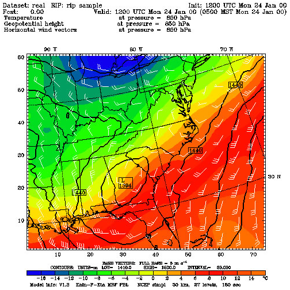
This FSG will generate 5 frames to create a single plot (as shown below):

· Temperature in degrees C (feld=tmc). This will be plotted as a horizontal contour plot (ptyp=hc), on pressure levels (vcor=p). The data will be interpolated to 850 hPa. The contour intervals are set to 2 (cint=2), and shaded plots (cmth=fill) will be generated with a color range from light violet to light gray.

· Geopotential heights (feld=ght) will also be plotted as a horizontal contour plot. This time the contour intervals will be 30 (cint=30), and contour lines with a line width of 2 (linw=2) will be used.

· Wind vectors (feld=uuu,vvv), plotted as barbs (vcmax=-1).

· A map background will be displayed (feld=map), and

· Tic marks will be placed on the plot (feld=tic).

Running RIP

Each execution of RIP requires three basic things: a RIP executable, a model data set and a user input file (UIF). The syntax for the executable, rip, is as follows:

rip [-f] model-data-set-name rip-execution-name

In the above, model-data-set-name is the same model-data-set-name that was used in creating the RIP data set with the program ripdp.

rip-execution-name is the unique name for this RIP execution, and it also defines the name of the UIF that RIP will look for.

The –f option causes the standard output (i.e., the textual print out) from RIP to be written to a file called rip-execution-name.out. Without the –f option, the standard output is sent to the screen.

e.g. rip -f RIPDP/arw rip_sample

If this is successful, the following files will be created:

rip_sample.TYPE - metacode file with requested plots
rip_sample.out - log file (if –f used) ; view this file if a problem occurred

The default output TYPE is a ‘cgm’, metacode file. To view these, use the command ‘idt’.

e.g. idt rip_sample.cgm

For high quality images, create pdf or ps images directly (ncarg_type = pdf / ps).

See the Tools section in Chapter 10 of this User’s Guide for more information concerning other types of graphical formats and conversions between graphical formats.

Examples of plots created for both idealized and real cases are available from:
http://www2.mmm.ucar.edu/wrf/users/graphics/RIP4/RIP4.htm

ARWpost

The ARWpost package reads-in WRF-ARW model data and creates GrADS output files. Since version 3.0 (released December 2010), vis5D output is no longer supported. More advanced 3D visualization tools, like VAPOR and IDV, have been developed over the last couple of years, and users are encouraged to explore those for their 3D visualization needs.

The converter can read-in WPS geogrid and metgrid data, and WRF-ARW input and output files in netCDF format. Since version 3.0 the ARWpost code is no longer dependant on the WRF IO API. The advantage of this is that the ARWpost code can now be compiled and executed anywhere without the need to first install WRF. The disadvantage is that GRIB1 formatted WRF output files are no longer supported.

Necessary software

GrADS software - you can download and install GrADS from http://grads.iges.org/. The GrADS software is not needed to compile and run ARWpost, but is needed to display the output files.

Obtain the ARWpost TAR file from the WRF Download page (http://www2.mmm.ucar.edu/wrf/users/download/get_source.html)

Unzip and untar the ARWpost tar file.

The tar file contains the following directories and files:

• README, a text file containing basic information on running ARWpost.
• arch/, directory containing configure and compilation control.
• clean, a script to clean compiled code.
• compile, a script to compile the code.
• configure, a script to configure the compilation for your system.
• namelist.ARWpost, namelist to control the running of the code.
• src/, directory containing all source code.
• scripts/, directory containing some grads sample scripts.
• util/, a directory containing some utilities.
  
  

Environment Variables

Set the environment variable NETCDF to the location where your netCDF libraries are installed. Typically (for cshrc shell):

setenv NETCDF /usr/local/netcdf

Configure and Compile ARWpost

To configure - Type:

./configure

You will see a list of options for your computer (below is an example for a Linux machine):


Will use NETCDF in dir: /usr/local/netcdf-pgi
-----------------------------------------------------------
Please select from among the following supported platforms.
1. PC Linux i486 i586 i686, PGI compiler
2. PC Linux i486 i586 i686, Intel compiler

Enter selection [1-2]

Make sure the netCDF path is correct.

Pick the compile option for your machine

 To compile - Type:

./compile

If successful, the executable ARWpost.exe will be created.

Edit the namelist.ARWpost file

Set input and output file names and fields to process (&io)

Variable	Value	Description
&datetime
start_date; end_date		Start and end dates to process. Format: YYYY-MM-DD_HH:00:00
interval_seconds	0	Interval in seconds between data to process. If data is available every hour, and this is set to every 3 hours, the code will skip past data not required.
tacc	0	Time tolerance in seconds. Any time in the model output that is within tacc seconds of the time specified will be processed.
debug_level	0	Set this higher for more print-outs that can be useful for debugging later.
&io
input_root_name	./	Path and root name of files to use as input. All files starting with the root name will be processed. Wild characters are allowed.
output_root_name	./	Output root name. When converting data to GrADS, output_root_name.ctl and output_root_name.dat will be created.
output_title	Title as in WRF file	Use to overwrite title used in GrADS .ctl file.
mercator_defs	.False.	Set to true if mercator plots are distorted.
split_output	.False.	Use if you want to split our GrADS output files into a number of smaller files (a common .ctl file will be used for all .dat files).
frames_per_outfile	1	If split_output is .True., how many time periods are required per output (.dat) file.
plot	‘all’	Which fields to process. ‘all’ – all fields in WRF file ‘list’ – only fields as listed in the ‘fields’ variable. ‘all_list’ – all fields in WRF file and all fields listed in the ‘fields’ variable. Order has no effect, i.e., ‘all_list’ and ‘list_all’ are similar. If ‘list’ is used, a list of variables must be supplied under ‘fields’. Use ‘list’ to calculate diagnostics.
fields		Fields to plot. Only used if ‘list’ was used in the ‘plot’ variable.
&interp
interp_method	0	0 - sigma levels, -1 - code-defined "nice" height levels, 1 - user-defined height or pressure levels
interp_levels		Only used if interp_method=1 Supply levels to interpolate to, in hPa (pressure) or km (height). Supply levels bottom to top.
extrapolate	.false.	Extrapolate the data below the ground if interpolating to either pressure or height.

Available diagnostics:

cape - 3d cape
cin - 3d cin
mcape - maximum cape
mcin - maximum cin

clfr - low/middle and high cloud fraction
dbz - 3d reflectivity
max_dbz - maximum reflectivity

geopt - geopotential
height - model height in km

lcl - lifting condensation level
lfc - level of free convection
pressure - full model pressure in hPa
rh - relative humidity
rh2 - 2m relative humidity
theta - potential temperature
tc - temperature in degrees C
tk - temperature in degrees K
td - dew point temperature in degrees C
td2 - 2m dew point temperature in degrees C

slp - sea level pressure

umet and vmet - winds rotated to earth coordinates
u10m and v10m - 10m winds rotated to earth coordinates
wdir - wind direction
wspd - wind speed coordinates
wd10 - 10m wind direction
ws10 - 10m wind speed 

Run ARWpost

Type:

./ARWpost.exe

This will create the output_root_name.dat and output_root_name.ctl files required as input by the GrADS visualization software.

NOW YOU ARE READY TO VIEW THE OUTPUT

For general information about working with GrADS, view the GrADS home page: http://grads.iges.org/grads/

To help users get started, a number of GrADS scripts have been provided:

· The scripts are all available in the scripts/ directory.

· The scripts provided are only examples of the type of plots one can generate with GrADS data.

· The user will need to modify these scripts to suit their data (e.g., if you do not specify 0.25 km and 2 km as levels to interpolate to when you run the "bwave" data through the converter, the "bwave.gs" script will not display any plots, since it will specifically look for these levels).

· Scripts must be copied to the location of the input data.

GENERAL SCRIPTS
cbar.gs	Plot color bar on shaded plots (from GrADS home page)
rgbset.gs	Some extra colors (Users can add/change colors from color number 20 to 99)
skew.gs	Program to plot a skewT TO RUN TYPE: run skew.gs (needs pressure level TC,TD,U,V as input) User will be prompted if a hardcopy of the plot must be created (- 1 for yes and 0 for no). If 1 is entered, a GIF image will be created. Need to enter lon/lat of point you are interested in Need to enter time you are interested in Can overlay 2 different times
plot_all.gs	Once you have opened a GrADS window, all one needs to do is run this script. It will automatically find all .ctl files in the current directory and list them so one can pick which file to open. Then the script will loop through all available fields and plot the ones a user requests.

SCRIPTS FOR REAL DATA
real_surf.gs	Plot some surface data Need input data on model levels
plevels.gs	Plot some pressure level fields Need model output on pressure levels
rain.gs	Plot total rainfall Need a model output data set (any vertical coordinate), that contain fields "RAINC" and "RAINNC"
cross_z.gs	Need z level data as input Will plot a NS and EW cross section of RH and T (C) Plots will run through middle of the domain
zlevels.gs	Plot some height level fields Need input data on height levels Will plot data on 2, 5, 10 and 16km levels
input.gs	Need WRF INPUT data on height levels

SCRIPTS FOR IDEALIZED DATA
bwave.gs	Need height level data as input Will look for 0.25 and 2 km data to plot
grav2d.gs	Need normal model level data
hill2d.gs	Need normal model level data
qss.gs	Need height level data as input. Will look for heights 0.75, 1.5, 4 and 8 km to plot
sqx.gs	Need normal model level data a input
sqy.gs	Need normal model level data a input

Examples of plots created for both idealized and real cases are available from:
http://www2.mmm.ucar.edu/wrf/OnLineTutorial/Graphics/ARWpost/

Trouble Shooting

The code executes correctly, but you get "NaN" or "Undefined Grid" for all fields
when displaying the data.

Look in the .ctl file.

a) If the second line is:

options byteswapped

Remove this line from your .ctl file and try to display the data again.
If this SOLVES the problem, you need to remove the -Dbytesw option from configure.arwp

b) If the line below does NOT appear in your .ctl file:

options byteswapped

ADD this line as the second line in the .ctl file.
Try to display the data again.
If this SOLVES the problem, you need to ADD the -Dbytesw option for configure.arwp

The line "options byteswapped" is often needed on some computers (DEC alpha as an example). It is also often needed if you run the converter on one computer and use another to display the data.  

NCEP Unified Post Processor (UPP)

UPP Introduction

The NCEP Unified Post Processor has replaced the WRF Post Processor (WPP). The UPP software package is based on WPP but has enhanced capabilities to post-process output from a variety of NWP models, including WRF-NMM, WRF-ARW, Non-hydrostatic Multi-scale Model on the B grid (NMMB), Global Forecast System (GFS), and Climate Forecast System (CFS). At this time, community user support is provided for the WRF-based systems and NMMB.

In addition to the option to output fields on the model’s native vertical levels, UPP interpolates output from the model’s native grids to National Weather Service (NWS) standard levels (pressure, height, etc.) and standard output grids (AWIPS, Lambert Conformal, polar-stereographic, etc.) in NWS and World Meteorological Organization (WMO) GRIB format. With the release of UPPv3.0, preliminary capabilities to output in GRIB Edition 2 (GRIB2) format for select models has been included and a simple template is available for users to modify to fit their needs. Caution should be taken when utilizing GRIB2; exhaustive testing has not been conducted and it is recommend to use this feature in testing/exploratory mode at this time. Updates will be provided as GRIB2 output capabilities become available and more comprehensive information will be included in the Users’ Guide.

UPP incorporates the Joint Center for Satellite Data Assimilation (JCSDA) Community Radiative Transfer Model (CRTM) to compute model derived brightness temperature (T_B) for various instruments and channels. This additional feature enables the generation of a number of simulated satellite products including GOES and AMSRE products for WRF-NMM, Hurricane WRF (HWRF), WRF-ARW and GFS. For CRTM documentation, refer to http://www.orbit.nesdis.noaa.gov/smcd/spb/CRTM.

UPP Software Requirements

The Community Unified Post Processor requires the same Fortran and C compilers used to build the WRF model. In addition, the netCDF library, the JasPer library, the PNG library, Zlib, and the WRF I/O API libraries, which are included in the WRF model tar file, are also required. UPP uses WRF I/O libraries for data processing of all models and as a result UPP is dependent on a WRF build. The JasPer library, PNG library, and Zlib are new requirements with the release of UPPv2.0 and higher, due to the addition GRIB2 capabilities. NCEP provides these necessary codes for download: http://www.nco.ncep.noaa.gov/pmb/codes/GRIB2/

The UPP has some sample visualization scripts included to create graphics using either GrADS (http://grads.iges.org/grads/grads.html) or GEMPAK (http://www.unidata.ucar.edu/software/gempak/index.html). These are not part of the UPP installation and need to be installed separately if one would like to use either plotting package.

UPP has been tested on LINUX platforms (with PGI, Intel and GFORTRAN compilers).

Obtaining the UPP Code

The UPP package can be downloaded from: http://www.dtcenter.org/upp/users/downloads/index.php

UPP Functionalities

The UPP,

· is compatible with WRF v3.3 and higher.

· can be used to post-process WRF-ARW, WRF-NMM, NMMB, GFS, and CFS forecasts (community support provided for WRF-based and NMMB forecasts).

· can ingest WRF history files (wrfout*) in two formats: netCDF and binary.

· can ingest NMMB history files (nmmb_hist*) in binary.

The UPP is divided into two parts:

Unipost

i. Interpolates the forecasts from the model’s native vertical coordinate to NWS standard output levels (e.g., pressure, height) and computes mean sea level pressure. If the requested parameter is on a model’s native level, then no vertical interpolation is performed.

ii. Computes diagnostic output quantities (e.g., convective available potential energy, helicity, relative humidity).

iii. Outputs the results in NWS and WMO standard GRIB1 format (for GRIB documentation, see http://www.nco.ncep.noaa.gov/pmb/docs/).

iv. Destaggers the WRF-ARW forecasts from a C-grid to an A-grid.

v. Outputs two navigation files, copygb_nav.txt (for WRF-NMM output only) and copygb_hwrf.txt (for WRF-ARW and WRF-NMM). These files can be used as input for copygb.

1. copygb_nav.txt: This file contains the GRID GDS of a Lambert Conformal Grid similar in domain and grid spacing to the one used to run the WRF-NMM. The Lambert Conformal map projection works well for mid-latitudes.

2. copygb_hwrf.txt: This file contains the GRID GDS of a Latitude-Longitude Grid similar in domain and grid spacing to the one used to run the WRF model. The latitude-longitude grid works well for tropics.

Copygb

1. Destaggers the WRF-NMM forecasts from the staggered native E-grid to a regular non-staggered grid. (Since unipost destaggers WRF-ARW output from a C-grid to an A-grid, WRF-ARW data can be displayed directly without going through copygb.)

2. Destaggers the NMMB forecasts from the staggered native B-grid to a regular non-staggered grid.

3. Interpolates the forecasts horizontally from their native grid to a standard AWIPS or user-defined grid (for information on AWIPS grids, see http://www.nco.ncep.noaa.gov/pmb/docs/on388/tableb.html).

4. Outputs the results in NWS and WMO standard GRIB1 format (for GRIB documentation, see http://www.nco.ncep.noaa.gov/pmb/docs/).

Full UPP documentation available at:

http://www.dtcenter.org/upp/users/docs/user_guide/V3/upp_users_guide.pdf

http://www.dtcenter.org/upp/users/index.php

VAPOR

VAPOR is the Visualization and Analysis Platform for Ocean, Atmosphere, and Solar Researchers. VAPOR was developed at NCAR to provide interactive visualization and analysis of numerically simulated fluid dynamics. The current (2.3) version of VAPOR has many capabilities for 3D visualization of WRF-ARW simulation output, including the ability to directly import wrfout files, and support for calculating derived variables that are useful in visualizing WRF output.

Basic capabilities of VAPOR with WRF-ARW output

· Direct Volume rendering (DVR)

Any 3D variable in the WRF data can be viewed as a density. Users control transparency and color to view temperature, water vapor, clouds, etc. in 3D.

· Flow

- Display barbs associated with 2D or 3D field magnitudes. Barbs can also be positioned at a specified height above the terrain and aligned to the WRF data grid.

- Draw 2D and 3D streamlines and flow arrows, showing the wind motion and direction, and how wind changes in time.

- Path tracing (unsteady flow) enables visualization of trajectories that particles take over time. Users control when and where the particles are released.

- Flow images (image based flow visualization) can be used to provide an animated view of wind motion in a planar section, positioned anywhere in the scene.

- Field line advection can be used to animate the motion of streamlines of any vector field in a moving wind field.

· Isosurfaces

The isosurfaces of variables are displayed interactively. Users can control iso-values, color and transparency of the isosurfaces. Isosurfaces can be colored according to the values of another variable.

· Contour planes and Probes

3D variables can be intersected with arbitrarily oriented planes. Contour planes can be interactively positioned. Users can interactively pinpoint the values of a variable and establish seed points for flow integration. Wind and other vector fields can be animated in the probe plane.

· Two-dimensional variable visualization

2D (horizontal) WRF variables can be color-mapped and visualized in the 3D scene. They can be viewed on a horizontal plane in the scene, or mapped onto the terrain surface.

· Animation

Control the time-stepping of the data, for interactive replaying and for recording animated sequences.

· Image display

Tiff images can be displayed in the 3D scene. If the images are georeferenced (i.e. geotiffs) then they can be automatically positioned at the correct latitude/longitude coordinates. Images can be mapped to the terrain surface, or aligned to an axis-aligned plane. Several useful georeferenced images are preinstalled with VAPOR, including political boundary maps, and the NASA Blue Marble earth image. VAPOR also provides several utilities for obtaining geo-referenced images from the Web. Images with transparency can be overlaid on the terrain images, enabling combining multiple layers of information.

· Analysis capabilities

VAPOR (versions 2.1+) has an embedded Python calculation engine. Derived variables can be easily calculated with Python expressions or programs and these will be evaluated as needed for use in visualization. VAPOR provides Python scripts to calculate the following variables from WRF output:

CTT: Cloud-top temperature

DBZ: 3D radar reflectivity

DBZ_MAX: radar reflectivity over vertical column

ETH: equivalent potential temperature

RH: relative humidity

PV: potential vorticity

SHEAR: horizontal wind hear

SLP: 2D sea-level pressure

TD: dewpoint temperature

TK: temperature in degrees Kelvin

Instructions for calculating and visualizing these and other variables are provided in the document, “Using Python with VAPOR” on the VAPOR website.

.

Derived variables can also be calculated in IDL and imported into the current visualization session. Variables can also be calculated in other languages (e.g. NCL) and adjoined to the Vapor Data Collection. Documentation of these capabilities can be found in the Documentation menu on the VAPOR website http://www.vapor.ucar.edu.

VAPOR requirements

VAPOR is supported on Linux, Mac, and Windows systems. VAPOR works best with a recent graphics card (say 1-2 years old). The advanced features of VAPOR perform best with nVidiaä, ATIä or AMDä graphics accelerators.

VAPOR is installed on NCAR visualization systems. Users with UCAR accounts can connect their (Windows, Linux or Mac) desktops to the NCAR visualization systems using NCAR’s VNC-based remote visualization services, to run VAPOR and visualize the results remotely. Instructions for using NCAR visualization services are at:

https://www2.cisl.ucar.edu/resources/geyser_caldera/visualization
Contact dasg@ucar.edu or vapor@ucar.edu for assistance.

VAPOR support resources

The VAPOR website: http://www.vapor.ucar.edu includes software, documentation, example data, and links to other resources. The document "Getting started with VAPOR and WRF"

(http://www.vapor.ucar.edu/docs/getting-started-vapor/getting-started-vapor-and-wrf) has an overview of the various capabilities that are useful in visualizing WRF data with VAPOR.

The VAPOR Sourceforge website (http://sourceforge.net/projects/vapor) enables users to post bugs, request features, download software, etc.

Users of VAPOR on NCAR visualization systems should contact dasg@ucar.edu for support.

Users are encouraged to provide feedback. Questions, problems, bugs etc. should be reported to vapor@ucar.edu. The VAPOR development priorities are set by users as well as by the VAPOR steering committee, a group of turbulence researchers who are interested in improving the ability to analyze and visualize time-varying simulation results.  Post a feature request to the VAPOR SourceForge website (http://sourceforge.net/projects/vapor), or e-mail vapor@ucar.edu if you have requests or suggestions about improving VAPOR capabilities.

Basic steps for using VAPOR to visualize WRF-ARW data

1. Install VAPOR
   
   

VAPOR installers for Windows, Macintosh and Linux are available on the VAPOR home page, http://www.vapor.ucar.edu/.

For most users, a binary installation is fine.  Installation instructions are also provided in the VAPOR documentation pages, http://www.vapor.ucar.edu/docs/install.

After VAPOR is installed, it is necessary to perform user environment setup on Unix or Mac, before executing any VAPOR software. These setup instructions are provided on the VAPOR binary install documentation pages:

http://www.vapor.ucar.edu/docs/install.

2. (Optional) Convert WRF output data to VAPOR Data Collection
   
   

Starting with VAPOR 2.0, you can directly load WRF-ARW output files into VAPOR. From the VAPOR menu select “Import data into current session---WRF-ARW”. Alternately, if your data is very large, you will be able to visualize it more interactively by converting it to a Vapor Data Collection (VDC).

A VAPOR VDC consists of (1) a metadata file (file type .vdf) that describes an entire VAPOR data collection, and (2) a directory of multi-resolution data files where the actual data is stored. The metadata file is created by the command wrfvdfcreate, and the multi-resolution data files are written by the command wrf2vdf. The simplest way to create a VAPOR data collection is using the vdcwizard application, which is installed with VAPOR. Also there are command-line tools wrfvdfcreate and wrf2vdf that can be used to convert the WRF-ARW output data to a VDC.

Using vdcwizard, you specify the name of the .vdf file and all the wrfout files that are to be used. First the .vdf file is created, then all the wrfout files are processed creating a VDC.

3. Visualize the WRF data

From the command line, issue the command “vaporgui”, or double-click the VAPOR desktop icon (on Windows or Mac). This will launch the VAPOR user interface.

To directly import WRF-ARW (NetCDF) output files, click on the Data menu, and select “Import WRF output files into default session”. Then select all the wrfout files you want to visualize and click “open”. If instead you converted your data to a VAPOR Data Collection, then, from the Data menu, choose “Load a dataset into default session”, and select the metadata file that you associated with your converted WRF data.

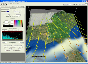
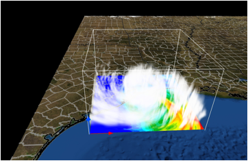
To visualize the data, select a renderer tab (DVR, Iso, Flow, 2D, Image, Barbs, or Probe), chose the variable(s) to display, and then, at the top of the tab, check the box labeled “Instance:1”, to enable the renderer. For example, the above top image combines volume, flow and isosurface visualization with a terrain image. The bottom image illustrates hurricane Ike, as it made landfall in 2008. The Texas terrain has a map of US Counties applied to it, and an NCL image of accumulated rainfall is shown at ground level in the current region.

4. Read the VAPOR Documentation

VAPOR documentation is provided on the Website http://www.vapor.ucar.edu. For a quick overview of capabilities of VAPOR with WRF data, see “Getting started with VAPOR and WRF”:

http://www.vapor.ucar.edu/docs/getting-started-vapor/getting-started-vapor-and-wrf.

A short tutorial, showing how to use VAPOR to visualize hurricane Katrina WRF output files, is provided at http://docs.vapor.ucar.edu/tutorials/hurricane-katrina.

Additional documents on the VAPOR website (http://www.vapor.ucar.edu) provide more information about visualization of WRF data. Information is also available in the VAPOR user interface to help users quickly get the information they need, and showing how to obtain the most useful visualizations. Note the following resources:

- The Georgia Weather Case Study

(http://www.vapor.ucar.edu/sites/default/files/docs/GeorgiaCaseStudy.pdf) provides a step-by-step tutorial, showing how to use most of the VAPOR features that are useful in WRF visualization. However this material is based on an older version of VAPOR.

- Creation of geo-referenced images to use with WRF data is discussed in the web document “Preparation of Georeferenced Images”.

(http://www.vapor.ucar.edu/docs/vapor-data-preparation/preparation-georeferenced-images)

- "Using NCL with VAPOR to visualize WRF-ARW data":

(http://www.vapor.ucar.edu/sites/default/files/docs/VAPOR-WRF-NCL.pdf)
is a tutorial that shows how to create geo-referenced images from NCL plots, and to insert them in VAPOR scenes.

- Fuller documentation of the capabilities of the VAPOR user interface is provided in the VAPOR GUI General Guide:

(http://www.vapor.ucar.edu/docs/vaporgui-help).

- The VAPOR Users' Guide for WRF Typhoon Research:

(http://www.vapor.ucar.edu/sites/default/files/docs/Typhoon.pdf)
provides a tutorial for using VAPOR on typhoon data, including instructions for preparing satellites images and NCL plots to display in the scene. This document is also fairly old.

To understand the meaning or function of an element in the VAPOR user interface:
Tool tips:  Place the cursor over a widget for a couple of seconds and a one-sentence description will be provided.

Context-sensitive help:  From the Help menu, click on “?Explain This”, and then click with the left mouse button on a GUI element, to obtain a longer technical explanation of the functionality.

Web help: From the vaporgui Help menu, various help topics associated with the current context can be selected. These will launch a Web browser displaying detailed information about the selected topic.