User’s Guide for Advanced Research WRF (ARW) Modeling System Version 2

Chapter 6: WRF-VAR

Table of Contents

• Introduction
• Goals Of This WRF-Var Tutorial 
• Tutorial Schedule
• Download Test Data
• The 3D-Var Observation Preprocessor (3DVAR_OBSPROC)
• Setting up WRF-Var
• Run WRF-Var CONUS Case Study
• WRF-Var Diagnostics
• Updating WRF lateral boundary conditions

Introduction

Data assimilation is the technique by which observations are combined with an NWP product (the first guess or background forecast) and their respective error statistics to provide an improved estimate (the analysis) of the atmospheric (or oceanic, Jovian, whatever) state. Variational (Var) data assimilation achieves this through the iterative minimization of a prescribed cost (or penalty) function. Differences between the analysis and observations/first guess are penalized (damped) according to their perceived error. The difference between three-dimensional (3D-Var) and four-dimensional (4D-Var) data assimilation is the use of a numerical forecast model in the latter.

MMM Division of NCAR supports a unified (global/regional, multi-model, 3/4D-Var) model-space variational data assimilation system (WRF-Var) for use by NCAR staff and collaborators, and is also freely available to the general community, together with further documentation, test results, plans etc., from the WRF 3D-Var web-page http://www.wrf-model.org/development/group/WG4. The documentation you are reading is the "Users Guide" for those interested in downloaded and running the code. This text also forms the documentation for the online tutorial. The online WRF-Var tutorial is recommended for people who are

· Potential users of WRF-Var who want to learn how to run WRF-Var by themselves;

· New users who plan on coming to the NCAR WRF-Var tutorial - for you we recommend that you try this tutorial before you come to NCAR whether you are able or unable to register for practice sessions, and this will hopefully help you to understand the lectures a lot better;

· Users who are looking for references to diagnostics, namelist options etc - look for 'Miscellanies' and 'Trouble Shooting' sections on each page.

If you are a new WRF-Var user, this tutorial is designed to take you through WRF-Var-related programs step by step. If you have familiar with 3/4D-Var systems, you may find useful information here too as the WRF-Var implementation of 3/4D-Var contains a number of unique capabilities (e.g. multiple background error models, WRF-framework based parallelism/IO, direct radar reflectivity assimilation). If you don't know anything about 3D-Var, you should first read the WRF-Var tutorial presentations available from the WRF 3D-Var web-page http://www.wrf-model.org/development/group/WG4.

Goals Of This WRF-Var Tutorial

In this WRF-Var tutorial, you will learn how to run the various components of the WRF-Var system. In the online tutorial, you are supplied with a test case including the following input data: a) observation file, b) WRF NETCDF background file (previous forecast used as a first guess of the analysis), and c) Background error statistics (climatological estimate of errors in the background file). In your own work, you will need to create these two input files yourselves.

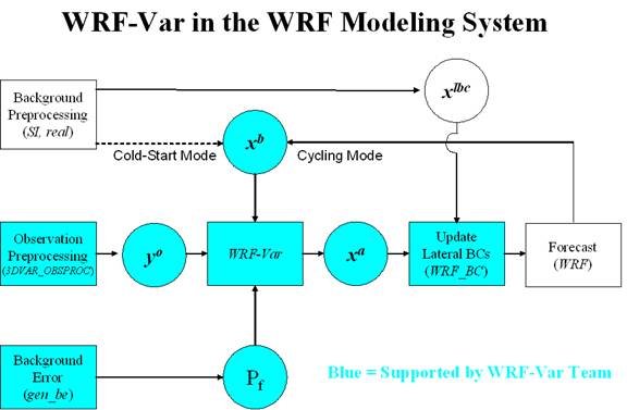
The components of the WRF-Var system are shown in blue in the sketch below, together with their relationship with rest of the WRF system.

Before using your own data, we suggest that you start by running through the WRF-Var related programs at least once using the supplied test case. This serves two purposes: First, you can learn how to run the programs with data we have tested ourselves, and second you can test whether your computer is adequate to run the entire modeling system. After you have done this tutorial, you can try

• Running other, more computationally intensive, case studies.

• Experimenting with some of the many namelist variables. WARNING: It is impossible to test every code upgrade with every permutation of computer, compiler, number of processors, case, namelist option, etc so please modify only those that are supported. The ones we support are indicated in the default run script (DA_Run_WRF-Var.csh). Good examples include withholding observations and tuning background error coefficients.

• Running with your own domain. Hopefully, our test cases will have prepared you (and us!) for the variety of ways in which you may wish to run WRF-Var. Please let us know your experiences.

As a professional courtesy, we request that you include the following reference in any publications that makes use of any component of the community WRF-Var system:

Barker, D. M., W. Huang, Y. R. Guo, and Q. N. Xiao., 2004: A Three-Dimensional (3DVAR) Data Assimilation System For Use With MM5: Implementation and Initial Results. Mon. Wea. Rev., 132, 897-914.

As you are going through the online tutorial, you will download program tar files and data to your local computer, compile and run on it. Do you know what machine you are going to use to run WRF-Var related programs? What compilers do you have on the machine?

Running WRF-Var requires a Fortran 90 compiler. We currently support the following platforms: IBM, DEC, SGI, PC/Linux (with Portland Group compiler), Cray-X1, and Apple G4/G5. Please let us know if this does not meet your requirements, and we will attempt to add other machines to our list of supported architectures as resources allow. Although we're interested to hear of your experiences modifying compile options, we do not yet recommend making changes to the configure file used to compile WRF-Var.

Tutorial Schedule

We recommend you follow the online tutorial in the order of the sections listed below. This tutorial does not cover parts of the larger WRF system, required if you wish to go beyond the test case supplied here, e.g. the WRF Standard Initialization (SI) and real pre-preprocessors are needed to create your own background field.

The online tutorial is broken down into the following sections.

a) Download Test Data: This page describes how to access test datasets to run WRF-Var.

b) The 3D-Var Observation Preprocessor (3DVAR_OBSPROC): Describes how to create an observation file for subsequent use in WRF-Var, and plot observation distributions.

c) Setting up WRF-Var: In this part of the tutorial you will download and compile the codes that form the WRF-Var system (3DVAR_OBSPROC, WRF-Var, WRF_BC).

d) Run WRF-Var CONUS Case Study: In this section, you will learn how to run WRF-Var for a test case.

e) WRF-Var Diagnostics: WRF-Var produces a number of diagnostics file that contain useful information on how the assimilation has performed. This section will introduce you to some of these files, and what to look for.

f) Updating WRF lateral boundary conditions: Before using the WRF-Var analysis as the initial conditions for a WRF forecast, the lateral boundary file must be modified to take account of the differences between first guess and analysis.

Download Test Data

This page describes how to access test datasets required to run WRF-Var. If you don't know anything about WRF-Var, you should first read the Introduction section.

Required Data

The WRF-Var system requires three input files to run: a) A WRF first guess input format file output from either the SI (cold-start) or WRF itself (warm-start), b) Observations (in BUFR or ASCII little_r format), and c) A background error statistics file (containing background error covariances currently calculated via the NMC-method). The use of these three data files in WRF-Var is described later in the tutorial.

The following table summarizes the above info:

Input Data	Format	Created By
First Guess	NETCDF	WRF Standard Initialization (SI) Or WRF
Observations	ASCII (BUFR also possible)	Observation Preprocessor (3DVAR_OBSPROC)
Background Error Statistics	Binary	WRF-Var gen_be utility

In the online tutorial, example input files are given. In your own work after the tutorial, you will need to create the input data sets yourselves.

Downloading Test Data

In the online tutorial, we will store data in a directory defined by the environment variable $DAT_DIR. This directory can be in any location that can be read and written to from your current machine and which have at least 100MB of memory available (for this test case, may be more for other cases).  Type

setenv DAT_DIR dat_dir

where dat_dir is your chosen directory. Create these directories (if they do not already exist) and type

cd $DAT_DIR

Download the tutorial test dataset for a CONUS 12 UTC 1 January 2003 test case from

http://www2.mmm.ucar.edu/individual/barker/wrfvar/wrfvar-testdata.tar.gz

Once you have downloaded the wrfvar-testdata.tar.gz file to $DAT_DIR, then extract it by typing

gunzip wrfvar-testdata.tar.gz

tar -xvf wrfvar-testdata.tar

You should then see a number of datafiles that will be used in the tutorial. To save space type

rm wrfvar-testdata.tar

What next?

OK, now you have downloaded the necessary data, you’re ready to preprocess the supplied observation file.

The 3D-Var Observation Preprocessor (3DVAR_OBSPROC)

By this stage you have successfully downloaded the test data for the tutorial and are ready to run 3DVAR observation preprocessor (3DVAR_OBSPROC).

Accessing and compiling the 3DVAR_OBSPROC code

First, go to your working directory and download the 3DVAR_OBSPROC code from

http://www2.mmm.ucar.edu/individual/barker/wrfvar/3DVAR_OBSPROC.tar.gz.

Once you have it on your machine, type the following to unzip and untar it:

gunzip 3DVAR_OBSPROC.tar.gz

tar -xvf 3DVAR_OBSPROC.tar

After this, you should see a directory 3DVAR_OBSPROC/ created in your working directory. If so remove the .tar file

rm 3DVAR_OBSPROC.tar

and cd to this directory:

cd 3DVAR_OBSPROC

Read the README file. To compile 3DVAR_OBSPROC, type

make

Once this is complete (a minute or less on most machines), you can check for the presence of the 3DVAR_OBSPROC executable by issuing the command (from the 3DVAR_OBSPROC directory)

ls -l src/3dvar_obs.exe

-rwxr-xr-x 1 mmm01 system 591184 May 29 2003 src/3dvar_obs.exe*

Running 3DVAR_OBSPROC

OK, so now you have compiled 3DVAR_OBSPROC. Before running the 3dvar_obs.exe, create the namelist file namelist.3dvar_obs and edit (see README.namelist for details);

cp namelist.3dvar_obs.wrfvar-tut namelist.3dvar_obs

then edit namelist.3dvar_obs.

In this tutorial, all you need to change is the full path to the observation file (ob.little_r) file, the grid dimensions (nestix=nestjx=45), and the resolution (dis=200[km]).

To run the 3DVAR_OBSPROC, type

3dvar_obs.exe >&! 3dvar_obs.out

Looking at 3DVAR_OBSPROC output.

Once the 3dvar_obs.exe has completed normally, you will have an observation data file: obs_gts.3dvar, which will be used as the input to WRF-Var. Before running WRF-Var, there is a utility to look at the data distribution for each type of observations.

1) cd MAP_plot;

2) Modify the shell script Map.csh to set the time window and full path of input observation file (obs_gts.3dvar);

3) Type

Map.csh

the configure.user will be automatically picked up for your computer system when you type Map.csh;

4) When the job has completed, you will have a gmeta file gmeta.{analysis_time}

which contains plots of data distribution for each type of observations contained in the OBS data file: obs_gts.3dvar. To view this, type

idt gmeta.2003010112

The gmeta file illustrates the geographic distribution of sonde observations for this case. You should see something like the following:

Saving necessary file for 3DVAR and clean 3DVAR_OBSPROC

In this tutorial, we are storing data in a directory defined by the environment variable $DAT_DIR. Having successfully created your own observation file (obs_gts.3dvar), copy it to $DAT_DIR using the command (from 3DVAR_OBSPROC directory)

mv obs_gts.3dvar $DAT_DIR/obs_gts.3dvar.2003010112

Finally, to clean up the 3DVAR_OBSPROC directory, type

make clean

Miscellanies:

1) When you run 3dvar_obs.exe, and you did not obtain the file obs_gts.3dvar, please check 3dvar_obs.out file to see where the program aborted. Usually there is information in this file to tell you what is wrong;

2) When you run 3dvar_obs.exe and got an error as 'Error in NAMELIST record 2' in 3dvar_obs.out file, please check if your namelist.3dvar_obs file matches with the Makefile settings. Either Your namelist.3dvar_obs file or Makefile need to be modified, then re-compile and re-run the job;

3) From the *.diag files, you may find which observation report caused the job failed;

4) In most cases, the job failed was caused by incorrect input files names, or the specified analysis time, time window, etc. in namelist.3dvar_obs;

5) If users still cannot figure out the troubles, please inform us and pass us your input files including the namelist file, and printed file 3dvar_obs.out.

What next?

OK, you have now created the observation file and looked at some plots of observations, now you are ready to move on to setting up WRF-Var.

Setting up WRF-Var

In this part of the tutorial you will download and compile the WRF-Var code. A description of the script that controls the running of WRF-Var and an overview of the namelist that it creates is also given.

Accessing WRF-Var code

First, go to your working directory and download the WRF-Var code from

http://www2.mmm.ucar.edu/individual/barker/wrfvar/wrfvar.tar.gz

Once you have it on your machine, type the following to unzip and untar it:

gunzip wrfvar.tar.gz

tar -xvf wrfvar.tar

After this, you should see a program directory wrfvar/ created in your working directory. If so, tidy up with the command

rm wrfvar.tar

cd to the wrfvar directory:

cd wrfvar

and you should see something like the following files and subdirectories listed (may be slightly different depending on version used):

ls -l

total 160

-rw-r--r-- 1 dmbarker users 15895 11 Jul 14:39 Makefile

-rw-r--r-- 1 dmbarker users 7189 4 Feb 07:40 README

-rw-r--r-- 1 dmbarker users 7263 11 Jul 14:39 README.NMM

-rw-r--r-- 1 dmbarker users 2548 18 Jan 2005 README_test_cases

drwxr-xr-x 3 dmbarker users 1024 27 Jul 08:55 Registry

drwxr-xr-x 3 dmbarker users 1024 27 Jul 08:55 arch

drwxr-xr-x 3 dmbarker users 1024 27 Jul 08:55 chem

-rwxr-xr-x 1 dmbarker users 1656 15 Apr 11:45 clean

-rwxr-xr-x 1 dmbarker users 7225 25 Jul 09:48 compile

-rwxr-xr-x 1 dmbarker users 10664 25 Jul 18:49 configure

drwxr-xr-x 7 dmbarker users 1024 27 Jul 08:55 convertor

drwxr-xr-x 6 dmbarker users 1024 27 Jul 08:55 da_3dvar

drwxr-xr-x 3 dmbarker users 1024 27 Jul 08:55 dyn_em

drwxr-xr-x 3 dmbarker users 1024 27 Jul 08:55 dyn_exp

drwxr-xr-x 3 dmbarker users 2048 27 Jul 08:55 dyn_nmm

drwxr-xr-x 14 dmbarker users 1024 27 Jul 08:55 external

drwxr-xr-x 3 dmbarker users 1024 27 Jul 08:55 frame

drwxr-xr-x 3 dmbarker users 1024 27 Jul 08:55 gen_be

drwxr-xr-x 3 dmbarker users 1024 27 Jul 08:55 inc

drwxr-xr-x 3 dmbarker users 1024 27 Jul 08:55 main

drwxr-xr-x 3 dmbarker users 2048 27 Jul 08:55 phys

drwxr-xr-x 4 dmbarker users 1024 27 Jul 08:56 run

drwxr-xr-x 3 dmbarker users 1024 27 Jul 08:55 scripts

drwxr-xr-x 3 dmbarker users 2048 27 Jul 08:55 share

drwxr-xr-x 12 dmbarker users 1024 27 Jul 08:55 test

drwxr-xr-x 4 dmbarker users 2048 27 Jul 08:55 tools

Compiling WRF-Var

To begin the compilation of WRF-Var, type the following to see the options available to you:

configure

You will then be queried with something like the following:

service01:>configure

option =

Please type : <configure var> to compile var,

or type : <configure be> to compile be.

The two choices refer to creating compiler options for WRF-Var, or alternatively to begin setting up the calculation of background error statistics. Here, we wish to compile WRF-Var, and so type

configure var

You will then see a list of alternative compilation options, depending on whether you want to run single processor, with different compilers etc, e.g.

option = var

configure var

checking for perl5... no

checking for perl... found /usr/local/bin/perl (perl)

Will use NETCDF in dir: /usr/local/netcdf

PHDF5 not set in environment. Will configure WRF for use without.

option = var

configure for var

------------------------------------------------------------------

Please select from among the following supported platforms.

1. Compaq OSF1 alpha (single-threaded)

2. Compaq OSF1 alpha DM (RSL, MPICH, RSL, IO)

3. Compaq OSF1 alpha (single-threaded, for compare with MM5 3DVAR)

Enter selection [1-3] :

In the online tutorial, you will be running WRF-Var in single processor mode. Therefore, enter 1 (single-threaded) at the prompt. This will automatically create a file configure.defaults_wrfvar in the wrfvar/arch subdirectory. This sets up compile options etc ready for compilation. We recommend you run WRF-Var in single processor mode first, but you later want to run WRF-Var on distributed memory machines to really speed things up.

Check the WRF-Var configure file has been produced by typing

ls -l arch/configure.defaults_wrfvar

Browse the file if interested, then to compile WRF-Var type

compile var

Once this is complete, you can check for the presence of the WRF-Var executable by issuing the command (from the wrfvar directory)

ls -l main/wrfvar.exe

-rwxr-xr-x   1 dmbarker users  11045892 May 29  2003 main/wrfvar.exe

While you are waiting for compilation to finish, we suggest you read the following sections to acquaint yourself with how you are going to run WRF-Var.

The DA_Run_WRF-Var.csh script.

The WRF-Var system is run (don’t do this yet in the online tutorial!) from the standard script wrfvar/run/DA_Run_WRF-Var.csh. An example ca be seen at

http://www2.mmm.ucar.edu/individual/barker/wrfvar/DA_Run_WRF-Var.csh.txt

The script performs a number of tasks, as follows:

a) Specify job details via environment variables: The user should be able, in most cases, to run WRF-Var just by resetting default environment variables (set below) to values for your particular application. Examples include changing data directory, filenames, and particular parameters within WRF (namelist.3dvar) and WRF (namelist.input) files.

b) Define default environment variables. These can be overridden in a) by setting non-default values.

c) Perform sanity checks (e.g. ensure input files exist). d) Create 3D-Var namelist file namelist.3dvar

d) Prepare for assimilation: link, and copy data/executables to the run directory.

e) Create namelist.3dvar and namelist.input files from environments specified above.

f) Run WRF-Var.

A brief description of the 3D-Var namelist options is now given.

The  WRF-Var namelist.3dvar file

There are many options you can change in a data assimilation system:  withholding particular observations, empirically retuning background errors, changing the minimization convergence criteria, etc, etc. To see the current full list of namelist options, check out the section of DA_Run_WRF-Var.csh that sets the default values. Not all values are provided with comments. This is deliberate – we only support changing the values with comments! Feel free to experiment with the others only if you can support yourself by checking the code to see what these other options do!

The namelist.3dvar file created for the tutorial case can be seen at

http://www2.mmm.ucar.edu/individual/barker/wrfvar/namelist.3dvar.txt

The  WRF namelist.input

Since WRF-Var is now a core for the WRF model, it uses the WRF framework to define and perform parallel, I/O functions. This is fairly transparent in the WRF-Var code. However, one disadvantage is that WRF-Var now requires one to specify the grid dimensions at run-time via a file (the previous serial version of MM5 3DVAR would pick these dimensions up from the input file and dynamically allocate memory).

For this tutorial, a 45x45x28 200km resolution case-study is used. These grid dimensions are specified via the default environment variables in the DA_Run_WRF-Var.csh script. You will need to change these values for your own domains.

The namelist.input file created for the tutorial case can be seen at

http://www2.mmm.ucar.edu/individual/barker/wrfvar/namelist.input.txt

What next?

Having compiled WRF-Var and familiarized yourself with the script and namelist files, it’s time to run WRF-Var!

Run WRF-Var CONUS Case Study

In this section, you will learn how to run WRF-Var using observations and a first guess from a low-resolution (200km) CONUS domain (see below).

By this stage you have successfully created the three input files (first guess, observation and background error statistics files in directory $DAT_DIR) required to run WRF-Var. Also, you have successfully downloaded and compiled the WRF-Var code. If this is correct, we are ready to learn how to run WRF-Var. If not, then you’ll need to return to stages a. to c.

The Case

The data for this case is valid at 12 UTC 1^st January 2003. The first guess comes from the NCEP global assimilation system (SSI), passed through the WRF Standard Initialization (SI) and real packages. The first-guess level 15 potential temperature field is shown below, illustrating the domain:

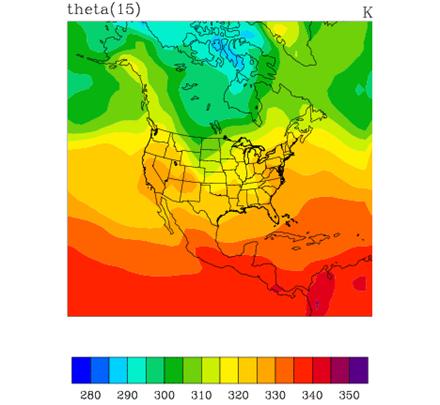
The intention of running this test-case is to provide a simplified, computationally cheap application in order to train potential uses of WRF-Var (this case uses only a small fraction of WRF-Var capabilities). To simplify the system further, only radiosonde observations are assimilated.

Required 3D-Var namelist changes

You will run WRF-Var using the script DA_Run_WRF-Var.csh found in subdirectory wrfvar/run. Open this script with your favorite editor, and spend some time browsing it to accustom yourself with the layout. Don’t despair, in this tutorial we will not be changing too much in here. See c. Setting Up WRF-Var for more information on the various namelist options.

In your first experiment, the only changes you need to make to the DA_Run_WRF-Var.csh script are to specify the DAT_DIR (input data directory) and WRFVAR_DIR (WRF-Var code directory) environment variables.

Run 3D-Var

Once you have set the necessary environment variables, run WRF-Var for this case study by typing

DA_Run_WRF-VAR.csh

in the wrfvar/run subdirectory.

Successful completion of the job results in a number of output diagnostics files in the ${RUN_DIR}/wrf-var subdirectory. The various textual diagnostics output files will be explained in the next section (WRF-Var Diagnostics). Here, we merely wish to run WRF-Var for this case.

In order to give yourself more experience with some of the 3D-Var options, try rerunning 3D-Var with different namelist.3dvar options. For example, making the WRF-Var convergence criteria more stringent by reducing the value of DA_EPS0 to e.g. 0.001. If WRF-Var has not converged by the maximum number of iterations (DA_NTMAX) then you may need to increase DA_NTMAX.

You may wish to change the RUN_DIR environment variable if you want to save all the outputs.

v. What next?

Having run WRF-Var, you should now spend time looking at some of the diagnostic output files created by WRF-Var.

WRF-Var Diagnostics

WRF-Var produces a number of diagnostics file that contain useful information on how the assimilation has performed. This section will introduce you to some of these files, and what to look for.

By this stage of the online tutorial you have successfully compiled and run WRF-Var.

Which are the important diagnostic to look for?

Having run WRF-Var, it is important to check a number of output files to see if the assimilation appears sensible. Change directory to where you ran the previous case-study:

cd ${RUN_DIR}/wrf-var

ls -l

You will see something like the following:

total 37990

-rwxr-xr-x 1 dmbarker users 10816316 27 Jul 19:43 wrfvar.exe

lrwxr-xr-x 1 dmbarker users 63 27 Jul 19:43 wrf_3dvar_input

-rw-r--r-- 1 dmbarker users 5508 27 Jul 19:43 namelist.input.txt

lrwxr-xr-x 1 dmbarker users 64 27 Jul 19:43 fort.92

lrwxr-xr-x 1 dmbarker users 47 27 Jul 19:43 fort.33

-rw-r--r-- 1 dmbarker users 2686 27 Jul 19:43 namelist.3dvar.txt

-rw-r--r-- 1 dmbarker users 8761 27 Jul 19:43 LANDUSE.TBL

-rw-r--r-- 1 dmbarker users 194 27 Jul 19:43 fort.82

-rw-r--r-- 1 dmbarker users 194 27 Jul 19:43 fort.81

-rw-r--r-- 1 dmbarker users 11848 27 Jul 19:43 fort.12

-rw-r--r-- 1 dmbarker users 5898 27 Jul 19:44 wrfvar.out

-rw-r--r-- 1 dmbarker users 4822312 27 Jul 19:44 wrf_3dvar_output

-rw-r--r-- 1 dmbarker users 158513 27 Jul 19:44 fort.60

-rw-r--r-- 1 dmbarker users 2827915 27 Jul 19:44 fort.50

-rw-r--r-- 1 dmbarker users 364 27 Jul 19:44 fort.48

-rw-r--r-- 1 dmbarker users 719125 27 Jul 19:44 fort.47

-rw-r--r-- 1 dmbarker users 194 27 Jul 19:44 DAProg_WRF_Var.grad_fn

-rw-r--r-- 1 dmbarker users 11848 27 Jul 19:44 DAProg_WRF-Var.statistics

-rw-r--r-- 1 dmbarker users 194 27 Jul 19:44 DAProg_WRF-Var.cost_fn

The most important output files here are

wrfvar.out: Text file containing information output as WRF-Var is running. Again, there is a host of information on number of observations, minimization, timings etc.

DAProg_WRF-Var.statistics: Text file containing O-B, O-A statistics (minimum, maximum, mean and standard deviation) for each observation type and variable. This information is very useful in diagnosing how WRF-Var has used different components of the observing system. Also contained are A-B statistics i.e. statistics of the analysis increments for each model variable at each model level. This information is very useful in checking the range of analysis increment values found in the analysis, and where they are in the grid.

fort.50: Data file containing detailed observation-based information for every observation, e.g. location, observed value, O-B, observation error, O-A, and quality control flag. This information is also used in a number of tuning programs found in the wrfvar/da_3dvar/utl directory.

wrf_3dvar_output: WRF (NETCDF) format file containing the analysis.

Take time to look through the textual output files to ensure you understand how 3DVAR has performed. For example,

How closely has WRF-Var fitted individual observation types? - Look in the DAProg_WRF-Var.statistics file to compare the O-B and O-A statistics.

How big are the analysis increments? Again, look in the DAProg_WRF-Var.statistics file to see minimum/maximum values of A-B for each variable.

How long did WRF-Var take to converge? Is it converged? Look in the wrfvar.out file, which will indicate the number of iterations taken by WRF-Var to converge. If this is the same as the maximum number of iterations specified in the namelist (DA_NTMAX) then you may need to increase this value to ensure convergence is achieved.

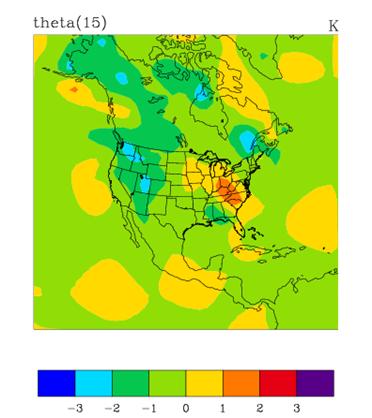
Plotting WRF-Var analysis increments

A good visual way of seeing the impact of assimilation of observations is to plot the analysis increments (i.e. analysis minus first guess difference). There are many different graphics packages used (e.g. RIP, NCL, GRADS etc) that can do this. The plot of level 15 theta increments below was produced using the particular NCL script wrftest.ncl. The plot indicates the magnitude, and scale of theta increments - the pattern is a function of observation distribution, observation minus first guess difference, and background error covariances used.

What next?

OK, you have run WRF-Var, checked out the diagnostics and are confident things are OK. Before running a forecast, you must first modify the tendencies within the lateral boundary condition files to be consistent with the new 3D-Var initial conditions.

Updating WRF lateral boundary conditions

Before running a forecast, you must first modify the tendencies within the lateral boundary condition files to be consistent with the new 3D-Var initial conditions. This is a simple procedure performed by the WRF utility WRF_BC.

Accessing the WRF_BC code

First, go to your working directory and download the WRF_BC code from

http://www2.mmm.ucar.edu/individual/barker/wrfvar/WRF_BC.tar.gz

Once you have it on your machine, type the following to unzip and untar it:

gunzip WRF_BC.tar.gz

tar -xvf WRF_BC.tar

After this, you should see a program directory WRF_BC/ created in your working directory. If so, tidy up with the command

rm WRF_BC.tar

cd to the WRF_BC directory:

cd WRF_BC

Compiling WRF_BC

The README file contains information on the role of WRF_BC, and how to compile. To do the latter, simply type

make

You will then see an executable by typing

ls -l update_wrf_bc.exe

Running WRF_BC

The update_wrf_bc.exe is run via the new_bc.csh script. Simply supply the names of the input analysis, lateral boundary condition, and WRF-Var analysis file names, The output can then be used as the initial conditions for WRF.

---

Once you are able to run all these programs successfully, and have spent some time looking at the variety of diagnostics output that is produced, we hope that you'll have some confidence in handling the WRF-Var system programs when you start your cases. Good luck!