User’s Guide for Advanced Research WRF (ARW) Modeling System Version 2
Chapter 8: Post-Processing Utilities
Table of Contents
· NCL
· RIP4
· ARWpost
· WPP
· Tools
Introduction
There are a number of visualization tools available to display WRF-ARW (http://wrf-model.org/) model data. Model data in netCDF format, can essentially be displayed using any tool capable of displaying this data format.
Currently the following post-processing utilities are supported, NCL, RIP4, ARWpost (converter to GrADS and Vis5D), and WPP.
NCL and RIP4 can currently only read data in netCDF format, while ARWpost can read data in netCDF and GRIB1 format, and WPP can read data in netCDF and binary format.
Required software:
The only library that is always required is the netCDF package from Unidata (http://www.unidata.ucar.edu/ : login > Downloads > NetCDF - registration login required).
netCDF stands for Network
Common Data Form. This format is
platform independent, i.e., data files can be read on both big_endian and
little_endian computers, regardless of where the file was created. To use the
netCDF libraries, ensure that the paths to these libraries are set correct in
your login scripts as well as all Makefiles.
Additional libraries required by each of the supported post-processing packages:
- NCL (http://www.ncl.ucar.edu/)
- GrADS (http://grads.iges.org/home.html)
- Vis5D (http://www.ssec.wisc.edu/~billh/vis5d.html)
-
GEMPAK (http://my.unidata.ucar.edu/content/software/gempak/index.html)
NCL
With the use of NCL Libraries (http://www.ncl.ucar.edu), WRF-ARW data can easily be displayed.
The information on these pages has been put together to help users generate NCL scripts to display their WRF-ARW model data.
Some example scripts are provided, but in order to fully utilize the functionality of the NCL Libraries, users should adapt these for their own needs, or write their own scripts.
NCL can process WRF ARW static/input and output files, as well as WRF-Var output data. Both single and double precision data can be processed.
What is NEW?
Up to July 2007, one
needed to install the NCL Libraries
(http://www.ncl.ucar.edu), AND the WRF_NCL package. (details’
regarding the old WRF_NCL package is available in Appendix B of this
User’s Guide).
In July 2007, the WRF_NCL package has been incorporated
into the NCL Libraries, thus only
the NCL Libraries, are now needed. NCL version 4.3.1 or higher is
required. (NOTE: some of the
built-in functions have been available since NCL version 4.3.0, but the
complete WRF-ARW package is only
available since version 4.3.1).
What has changed?
- The basic functions / procedures used in WRF_NCL has been moved in under the NCL libraries and are now located in "$NCARG_ROOT/lib/ncarg/nclscripts/wrf/".
- All the FORTRAN subroutines used for diagnostics and interpolation (previously located in wrf_user_fortran_util_0.f) has been re-coded into NCL in-line functions. This means a user no longer need to compile these.
What is NCL
The NCAR Command Language (NCL) is a free interpreted language designed specifically for scientific data processing and visualization. NCL has robust file input and output. It can read in netCDF, HDF4, HDF4-EOS, GRIB, binary and ASCII data. The graphics are world class and highly customizable.
It runs on many different operating systems including
Solaris, AIX, IRIX, Linux, MacOSX, Dec Alpha, and Cygwin/X running on Windows.
The NCL binaries are freely available at:
http://www.ncl.ucar.edu/Download/
To read more about NCL, please visit: http://www.ncl.ucar.edu/overview.shtml
Necessary software
NCL libraries (version 4.3.1 or higher).
.hlureasfile
Create a file called .hluresfile in your $HOME
directory. This file controls the color / background / fonts and basic size of
your plot. For more information regarding this file, see: http://www.ncl.ucar.edu/Document/Graphics/hlures.shtml.
NOTE: This file must reside in your $HOME
directory and not where you plan on running NCL.
Below is the .hluresfile used in the example scripts posted on the web (scripts are available at, http://www2.mmm.ucar.edu/wrf/users/graphics/NCL/NCL.htm). If a different color table is used, the plots will appear different. Copy the following to your ~/.hluresfile. (A copy of this file is available at, http://www2.mmm.ucar.edu/wrf/users/graphics/NCL/.hluresfile)
*wkColorMap
: WhViBlGrYeOrReWh
*wkBackgroundColor
: white
*wkForegroundColor
: black
*FuncCode
: ~
*TextFuncCode
: ~
*Font
: helvetica
*wkWidth
: 900
*wkHeight
: 900
NOTE: If your image has a black background with white lettering, your .hluresfile has not been created correctly, or it is in the wrong location.
Create NCL scripts
The basic outline of any NCL
script will look as follows:
|
load external functions and
procedures begin ; Open input file(s) ; Open graphical output ; Read variables ; Set up plot resources & Create plots ; Output graphics end |
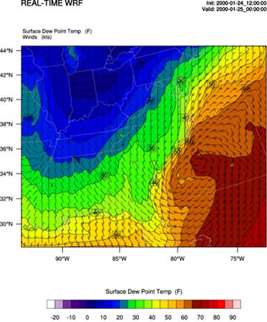
For example, let’s create a script to plot Temperature and Wind as shown in the picture below.
|
; load functions and
procedures load
"$NCARG_ROOT/lib/ncarg/nclscripts/csm/gsn_code.ncl" load
"$NCARG_ROOT/lib/ncarg/nclscripts/wrf/WRFUserARW.ncl" begin ; WRF ARW input file a
= addfile("../wrfout_d01_2000-01-24_12:00:00.nc","r") ; Output on screen. Output
will be called "plt_Surface1" type
= "x11" wks
= gsn_open_wks(type,"plt_Surface1") ; Set basic options ; Give our plot a main
title ; Set Footers off ARWres
= True ARWres@MainTitle
= "REAL-TIME WRF" ARWres@Footer
= False ;---------------------------------------------------------------
; Lets find out how many
times are in the datasets. times
= wrf_user_list_times(a) ; get times in the file ntimes
= dimsizes(times) ; number of times in the file it
= ntimes-1 ; we are only interested in the last time ARWres@TimeLabel
= times(it) ; keep some time information
; Create a MAP background mpres
= True map
= wrf_map(wks,a,mpres) ;--------------------------------------------------------------- ; Get variables tc2
= wrf_user_getvar(a,"T2",it) ; Get T2 (deg K) tc2
= tc2-273.16 ; Convert to deg C tf2
= 1.8*tc2+32. ; Turn temperature into Fahrenheit
tf2@description = "Surface Temperature"
tf2@units = "F" td_f = 1.8*td2+32. u10
= wrf_user_getvar(a,"U10",it) ; Get U10 v10
= wrf_user_getvar(a,"V10",it) ; get V10 u10
= u10*1.94386 ; Turn wind into knots v10
= v10*1.94386
u10@units = "kts"
v10@units = "kts" ;---------------------------------------------------------------
opts
= ARWres opts@cnFillOn
= True ; Shaded plot opts@ContourParameters
= (/ -20., 90., 5./) ; Contour intervals opts@gsnSpreadColorEnd
= -3 ; End 3rd from last color contour_tc
= wrf_contour(a,wks,tf2,opts) ; Create plot delete(opts)
; Plotting options for
Wind Vectors opts
= ARWres opts@FieldTitle
= "Winds" ; Overwrite the field title opts@NumVectors
= 47 ; Density of wind barbs - high is denser vector
= wrf_vector(a,wks,u10,v10,opts); Create plot delete(opts) ; MAKE PLOTS wrf_map_overlay(wks,map,(/contour_tc,contour_psl,vector/),True)
;--------------------------------------------------------------- end |
Extra sample scripts are available at, http://www2.mmm.ucar.edu/wrf/users/graphics/NCL/NCL.htm
Run NCL scripts
ncl NCL_script
The output created with this
command is controlled by the line:
wks = gsn_open_wk (type,"Output") inside the NCL script
where type can be x11, pdf, ncgm, ps, eps
Miscellaneous
For high quality images, create pdf / ps or eps images
directly via the ncl scripts (type = pdf / ps / eps)
See the Tools
section at the end of this chapter for more information concerning other types
of graphical formats and conversions between graphical formats.
Functions / Procedures under "$NCARG_ROOT/lib/ncarg/nclscripts/wrf/"
WRFUserARW.ncl
These functions and procedures are described fully on the
NCL web site (http://www.ncl.ucar.edu/Document/Functions/WRF_arw).
-
Controls plotting options. If you want to change the
defaults, change them in your script.
e.g., if you do not want footers at the bottom of your plots, set "res@Footer=False".
|
MainTitlePos |
Options are top "Left", "Center", "Right" |
|
InitTime |
Add Initial Time to plot |
|
ValidTime |
Add Valid Time to Plot |
|
TimePos |
Placement of Time Information. Options are top "Left" or "Right". If MainTitlePos and TimePos are on same side, Time Information will be plotted under the Main Title |
|
Footer |
Add some model information as a Footer to the plots |
- Controls map plotting, creation of plots and overlays, via the following functions:
wrf_contour
wrf_vector
wrf_map
wrf_map_zoom
wrf_map_overlay
wrf_overlay
-
Get variables from wrf files (wrf_user_getvar)
- Calculate diagnostics
All diagnostics are in-line functions
within NCL (http://www.ncl.ucar.edu/Document/Functions/wrf.shtml)
.
These functions can be used directly
inside any NCL script without the use of the WRFUserARW.ncl script, but it is
recommended to use the interface script, as this will make the use of these
functions much easier.
-
Interpolate data horizontally and vertically (wrf_user_intrp3d)
-
Obtain x/y locations for given lat/long locations (wrf_user_latlon_to_ij)
-
Extract times from wrf files (wrf_user_list_times)
Adding diagnostics using FORTRAN code
It is possible to link your favorite FORTRAN diagnostics routines to NCL. The only requirement is that the code must be written in FORTRAN 77. NCL does not recognize FORTRAN 90 code.
Let’s use a routine that calculated temperature (K) from theta and pressure. Add the markers NCLFORTSTART and NCLEND to the subroutine as indicated below. Note, that local variables are outside these block markers.
|
C NCLFORTSTART subroutine
compute_tk (tk,pressure,theta, nx, ny,
nz) C Variables integer nx,ny,nz real tk(nx,ny,nz) C NCLEND
C Local Variables integer i,j,k DO k=1,nz ENDDO |
Now compile this code using the NCL script WRAPIT.
WRAPIT
myTK.f
If WRAPIT cannot be found, make sure the environment variable NCARG_ROOT has been set correctly.
If the subroutine compiles successfully, a new library will be created, called myTK.so. This library can be linked to an NCL script to calculate TK. See how this is done in the example below:
|
load "$NCARG_ROOT/lib/ncarg/nclscripts/csm/gsn_code.ncl" load
"$NCARG_ROOT/lib/ncarg/nclscripts/wrf/WRFUserARW.ncl” begin t =
wrf_user_getvar(a,”T”,5) p =
wrf_user_getvar(a,”pressure”,5) dim = dimsizes(t) tk = new( (/ dim(0), dim(1), dim(2) /),
float) myTK :: compute_tk (tk,p,t,dim(2),dim(1),dim(0)) end |
RIP4
RIP4 was adapted from the RIP code, originally developed to
display MM5 model data. (Developed primarily by Mark Stoelinga, from both
NCAR and the
The RIP users' guide (http://www2.mmm.ucar.edu/wrf/users/docs/ripug.htm) is essential reading.
Code history
Version 4.0: reads WRF-ARW real output files
Version 4.1: reads idealized WRF-ARW datasets
Version 4.2: reads all the files produced by WPS
Version 4.3: reads files produced by WRF-NMM model (This document will only concentrate on running RIP4 for WRF-ARW. For
details on running RIP4 for WRF-NMM, see the WRF-NMM User’s Guide: http://www.dtcenter.org/wrf-nmm/users/docs/user_guide/WPS/index.php)
Necessary software
Obtain the RIP4 TAR file from the WRF Download page (http://www2.mmm.ucar.edu/wrf/users/download/get_source.html)
RIP4 only
requires low level NCAR Graphics libraries. These libraries has been merged
with the NCL libraries since the release of NCL version 5 (http://www.ncl.ucar.edu/),
so if you don’t already have NCAR Graphics installed on your computer,
install NCL.
Hardware
The code has been ported to: DEC Alpha, Linux (pgi and intel compilers). MAC (xlf and absoft compilers), SUN, SGI, IBM, CRAY and Fujitsu computers.
Steps to compile and run
Unzip and untar RIP4.TAR.gz file
Inside the TAR file you will see the following files:
CHANGES
Doc/
Makefile
README
color.tbl
psadilookup.dat
sample_infiles/ | sample scripts moved under this directory
in version 4.3
src/
stationlist
Compile the code
Typing "make" will produce the following list of compile options
|
make dec make linux make intel make sun make sun2 make sun90 make sgi make sgi64 make ibm make cray make vpp300 make vpp5000 make clean make clobber |
To Run on DEC_ALPHA To Run on LINUX with PGI compiler To Run on LINUX with INTEL compiler To Run on MAC_OS_X with Xlf Compiler To Run on MAC_OS_X
with Absoft Compiler To Run on SUN To Run on SUN if make sun didn't work To Run on SUN usingF90 To Run on SGI To Run on 64-bit SGI To Run on IBM SP2 To Run on NCAR's Cray To Run on Fujitsu VPP 300 To Run on Fujitsu VPP 5000 to remove object files to remove object files and executables |
Pick the compiler option for the machine you are working on
and type:
"make machine"
e.g. make linux
will compile the code for a Linux computer running PGI compiler
After a successful compilation, the following
new files should be created.
|
rip |
RIP post-processing program. |
|
ripcomp |
This program reads in two rip data files and compares their contents. |
|
ripdp_mm5 |
RIP Data Preparation program for MM5 data |
|
ripdp_wrfarw |
RIP Data Preparation program for WRF data |
|
ripinterp |
This program reads in model output (in rip-format files) from a coarse domain and from a fine domain, and creates a new file which has the data from the coarse domain file interpolated (bi-linearly) to the fine domain. The header and data dimensions of the new file will be that of the fine domain, and the case name used in the file name will be the same as that of the fine domain file that was read in. |
|
ripshow |
This program reads in a rip data file and prints out the contents of the header record. |
|
showtraj |
Sometimes, you may want to examine the contents of a trajectory position file. Since it is a binary file, the trajectory position file cannot simply be printed out. showtraj, reads the trajectory position file and prints out its contents in a readable form. When you run showtraj, it prompts you for the name of the trajectory position file to be printed out. |
|
tabdiag |
If fields are specified in the plot specification table for a trajectory calculation run, then RIP produces a .diag file that contains values of those fields along the trajectories. This file is an unformatted Fortran file; so another program is required to view the diagnostics. tabdiag serves this purpose. |
|
upscale |
This program reads in model output (in rip-format files) from a coarse domain and from a fine domain, and replaces the coarse data with fine data at overlapping points. Any refinement ratio is allowed, and the fine domain borders do not have to coincide with coarse domain grid points. |
Prepare the data
To prepare the data for the RIP program, one much first run RIPDP (RIP Data Preparation), for WRF (i.e., either ripdp_wrfarw or ripdp_wrfnmm depending on the core used
when running the WRF model).
As this step will create a large number of extra files, creating a new directory to place these files in, will enable you to manage the files easier
mkdir RIPDP
Edit the namelist sample_infiles /ripdp_wrfarw_sample.in (the
use of this namelist is optional). The most important information needed in
the namelist, is the times you want to process.
Run ripdp for WRF-ARW
ripdp_wrfarw [-n
namelist_file] casename [basic|all]
input1 input2 …
e.g. ripdp_wrfarw RIPDP/arw
all
../wrfout_d01_2000-01-24_12:00:00
>& ripdp_log
Check the ripdp_log for run time errors.
Edit the User Input File
The first step in creating the graphics you are interested
in, is to edit the User Input File (UIP)
sample_infiles /rip_sample.in (or
create your own UIP)
The UIP file consists of:
- 2 namelists: userin (which control the general input specifications) and trajcalc (which control the creation of trajectories); and
-
the Plot Specification Table (PST), used to control the generation of
the graphics
namelist: userin
|
Variable |
Type |
Description |
|
idotitle |
Integer |
Control first part of title line. |
|
titlecolor |
Character |
Control color of the title lines |
|
ptimes |
Integer |
Times to process. |
|
ptimeunits |
Character |
Time units. |
|
tacc |
Real |
Time tolerance in seconds. |
|
timezone |
Integer |
Specifies the offset from Greenwich time. |
|
iusdaylightrule |
Integer |
Flag to determine if |
|
iinittime |
Integer |
Controls the plotting of the initial time on the plots. |
|
ivalidtime |
Integer |
Controls the plotting of the plot valid time. |
|
inearesth |
Integer |
Plot time as two digits rather than 4 digits. |
|
flmin |
Real |
Left frame limit |
|
flmax |
Real |
Right frame limit |
|
fbmin |
Real |
Bottom frame limit |
|
ftmax |
Real |
Top frame limit |
|
ntextq |
Integer |
Quality of the text |
|
ntextcd |
Integer |
Text font |
|
fcoffset |
Integer |
Change initial time to something other than output initial time. |
|
idotser |
Integer |
Generate time series output files (no plots) only ASCII file that can be used as input to a plotting program). |
|
idescriptive |
Integer |
Use more descriptive plot titles. |
|
icgmsplit |
Integer |
Split metacode into several files. |
|
maxfld |
Integer |
Reserve memory for RIP. |
|
ittrajcalc |
Integer |
Generate trajectory output files (use namelist trajcalc when this is set). |
|
imakev5d |
Integer |
Generate output for Vis5D |
Plot Specification Table
The second part of the RIP UIF consists of the Plot Specification Table. The
PST provides all of the user control over particular aspects of individual frames
and overlays.
The basic structure of the PST is as follows:
- The first line of the PST is a line of consecutive equal signs. This line as well as the next two lines is ignored by RIP, it is simply a banner that says this is the start of the PST section.
- After that there are several groups of one or more lines separated by a full line of equal signs. Each group of lines is a frame specification group (FSG), and it describes what will be plotted in a single frame of metacode. Each FSG must end with a full line of equal signs, so that RIP can determine where individual frames starts and ends.
-
Each line within a FGS is referred to as a plot
specification line (PSL). A FSG that consists of three PSL lines will result in
a single metacode frame with three overlaid plots.
|
Example of a frame
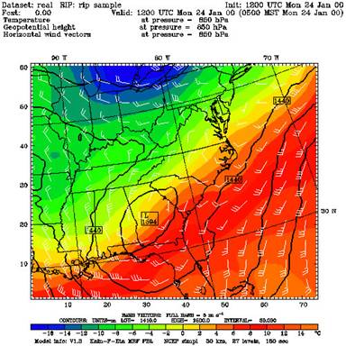
specification groups (FSG's): ============================================== feld=tmc;
ptyp=hc; vcor=p; levs=850; > cint=2; cmth=fill;
cosq=-32,light.violet,-24, 16,orange,24,brown,32,light.gray feld=ght;
ptyp=hc; cint=30; linw=2 feld=uuu,vvv; ptyp=hv; vcmx=-1; colr=white;
intv=5 feld=map;
ptyp=hb feld=tic;
ptyp=hb =============================================== |
This FSG will generate 5 frames to create a single plot (as shown below):
- Temperature in degrees C (feld=tmc). This will be plotted as a horizontal contour plot (ptyp=hc), on pressure levels (vcor=p). The data will be interpolated to 850 hPa. The contour intervals are set to 2 (cint=2), and shaded plots (cmth=fill) will be generated with a color range from light violet to light gray.
- Geopotential heights (feld=ght) will also be plotted as a horizontal contour plot. This time the contour intervals will be 30 (cint=30), and contour lines, with a line width of 2 (linw=2) will be used.
- Wind vectors (feld=uuu,vvv), plotted as barbs (vcmax=-1).
- A map background will be displayed (feld=map), and
- Tic marks will be placed on the plot (feld=tic).
Create graphics
First set the environment variables:
setenv NCARG_ROOT your_ncarg_location [typically /usr/local/ncarg]
setenv RIP_ROOT your_rip4_directory
Run rip
rip [-f] model_case_name rip_case_name
e.g. rip -f
RIPDP/arw rip_sample
If this is successful, the following files will be created
rip_sample.cgm gmeta file
rip_sample.out log file - view this file if a
problem occurred
View the meta file
To view the meta file, use the command "idt", e.g.
idt rip_sample.cgm
Examples of plots created for both idealized and real cases
are available from:
http://www2.mmm.ucar.edu/wrf/users/graphics/RIP4/RIP4.htm
Miscellaneous
See the Tools section at
the end of this chapter for more information concerning other types of
graphical formats and conversions between graphical formats.
ARWpost
The ARWpost package reads in WRF-ARW model data and creates output in either GrADS or Vis5D format.
The converter can read in WPS geogrid and metgrid data, and WRF-ARW input and output files.
The package makes use of the WRF IO API. The netCDF format has been tested extensively. GRIB1 format has been tested, but not as extensively. BINARY data cannot be read at the moment.
Necessary software
Obtain the ARWpost TAR file from the WRF Download page (http://www2.mmm.ucar.edu/wrf/users/download/get_source.html)
WRFV2 must be installed and available somewhere, as ARWpost
makes use of the common IO API libraries from WRFV2.
GrADS software - You can download and install GrADS
from http://grads/iges.org/grads. The GrADS
software is not needed to compile and run ARWpost.
Vis5D software (http://www.ssec.wisc.edu/~billh/vis5d.html)
Vis5D libraries must be installed to compile and run the ARWpost code, when creating Vis5D input data. If Vis5D files are not being created, these libraries are NOT needed to compile and run ARWpost.
Hardware
The code has been ported to the following machines
DEC Alpha , Linux (PGI and INTEL compilers) , MAC (with xlf compilers), SUN, SGI, IBM
Steps to compile and run
Untar ARWpost TAR file
Inside the TAR file you will have the following files:
|
README |
|
|
arch/ clean* compile* configure* |
Configure and compilation control |
|
namelist.ARWpost |
namelist |
|
fields.plt myLIST |
Samples to illustrate how to add fields to
plot via a file |
|
src/ |
Source code
|
|
scripts/ |
Sample scripts |
|
gribinfo.txt gribmap.txt |
Files
needed to process GRIB1 data. Do not edit these files |
|
util/ |
Utility
program |
Configure
WRFV2 must be compiled and available on your system.
Type: ./configure
You will see a list of options for your computer (below is an
example for a Linux machine)
Will use NETCDF in dir:
/usr/local/netcdf-pgi
-----------------------------------------------------------
Please select from among the following supported platforms.
1. PC Linux i486 i586 i686, PGI compiler (no vis5d)
2. PC Linux i486 i586 i686, PGI compiler (vis5d)
3. PC Linux i486 i586 i686, Intel compiler (no vis5d)
4. PC Linux i486 i586 i686, Intel compiler (vis5d)
Enter selection [1-4]
Make sure the netCDF path is correct.
Pick compile options for your machine (if you do not have Vis5D, or if you do not plan on using it, pick an option without Vis5D libraries)
Compile
If your WRFV2 code is NOT compiled under ../WRFV2, edit configure.arwp, and set "WRF_DIR" to the correct location of your WRFV2 code.
Type:
./compile
This will create the ARWpost.exe executable.
Edit the namelist.ARWpost file
Set times to process (&datetime)
Set input and output file names and fields to process (&io)
|
io_form_input |
2=netCDF, 5=GRIB1 |
|
input_root_name |
Path and root name of files to use as input. All files starting with the root name will be processed. Do not use wild characters in the input_root_name. |
|
output_root_name |
Output root name. When converting data to GrADS, output_root_name.ctl and output_root_name.dat will be created. For Vis5D, output_root_name.v5d will be created. |
|
plot |
Which fields to process. |
|
fields |
Fields to plot. Only used is list was used in the “plot” variable. |
|
fields_file |
File name that contains list of fields to plot. Only used is file was used in the “plot” variable. |
|
output_type |
Options are 'grads' (default) or 'v5d'
|
|
mercator_defs |
Set to true if mercator plots are distorted |
Available diagnostics: height (model height in km), theta (potential temperature), tc (temperature in degrees C), tk (temperature in degrees K), td (dew point temperature in degrees C), rh (relative humidity), pressure (full model pressure in hPa), dbz (3d reflectivity), max_dbz (maximum reflectivity), slp (sea level pressure), mcape (maximum CAPE), mcin (maximum CIN), lcl (lifting condensation level), lfc (level of free convection), cape (3d CAPE), cin (3d CIN), umet and vmet (winds rotated to earth coordinates), u10m and v10m (10m winds rotated to earth coordinates), wdir (wind direction), wspd (wind speed)
Set levels to interpolate too (&interp)
interp_method: 0=sigma levels,
-1=code defined "nice" height levels, 1=user defined height or
pressure levels
interp_levels: Only used if interp_method=1
Supply levels to interpolate to, in
hPa (pressure) or km (height)
Supply levels bottom to top
For extra information regarding the namelist.ARWpost file, refer to the README file.
Run
Type: ./ARWpost.exe
This will create output_root_name.dat and output_root_name.ctl
files if creating GrADS input, and output_root_name.v5d, if creating Vis5D input.
NOW YOU ARE READY TO VIEW THE OUTPUT
GrADS
For general information about working with GrADS, view the GrADS home page: http://grads.iges.org/grads/
To help users get started a number of GrADS scripts have been provided:
- The scripts are all available in the scripts/ directory.
- The scripts provided are only examples of the type of plots one can generate with GrADS data.
- The user will need to modify these script to suit their data (e.g., if you did not specify 0.25 km and 2 km as levels to interpolate to when you run the "bwave" data through the converter, the "bwave.gs" script will not display any plots, since it will specifically look for these to levels).
- Scripts must be copied to the location of the input data.
|
GENERAL SCRIPTS |
|
|
|
|
|
cbar.gs |
Plot color bar on shaded plots (from GrADS home page) |
|
rgbset.gs |
Some extra colors (Users can add/change colors from color number 20 to 99) |
|
skew.gs |
Program to plot a skewT |
|
plotALL.gs |
Once you have opened a GrADS window, all one needs to do is run this script. It will automatically find all .ctl files in the current directory and list them so one can pick which file to open. Then the script will loop through all available fields and plot the ones a user requests. |
-
|
SCRIPTS FOR REAL
DATA |
|
|
|
|
|
real_surf.gs |
Plot some surface data |
|
plevels.gs |
Plot some pressure level fields |
|
rain.gs |
Plot total rainfall |
|
cross_z.gs |
Need z level data as input |
|
zlevels.gs |
Plot some height level fields |
|
input.gs |
Need WRF INPUT data on height levels |
-
|
SCRIPTS FOR
IDEALIZED DATA |
|
|
|
|
|
bwave.gs |
Need height level data as input |
|
grav2d.gs |
Need normal model level data |
|
hill2d.gs |
Need normal model level data |
|
qss.gs |
Need height level data as input. |
|
sqx.gs |
Need normal model level data a input |
|
sqy.gs |
Need normal model level data a input |
Examples of plots created for both idealized and real cases
are available from:
http://www2.mmm.ucar.edu/wrf/users/graphics/ARWpost/ARWpost.htm
Trouble Shooting
The code executes correctly, but you get "NaN"
or "Undefined
Grid" for
all fields
when displaying the data.
Look in the .ctl file.
a) If the second line is:
options byteswapped
Remove this line from your .ctl file and try to display the data again.
If this SOLVES the problem, you need to remove the -Dbytesw
option from configure.arwp
b) If the line below does NOT appear in your .ctl file:
options byteswapped
ADD this line as the second line in the .ctl file.
Try to display the data again.
If this SOLVES the problem, you need to ADD the -Dbytesw option for
configure.arwp
The line "options byteswapped" is often needed on some computers (DEC alpha as an example). It is also often needed if you run the converter on one computer and use another to display the data.
Vis5D
For general information about working with Vis5D, view the Vis5D home page: http://www.ssec.wisc.edu/~billh/vis5d.html
WPP
The NCEP
WRF Postprocessor was designed to interpolate both WRF-ARW and WRF-NMM output
from their native grids to National Weather Service (NWS) standard levels (pressure, height, etc.) and standard output
grids (AWIPS, Lambert Conformal,
polar-stereographic, etc.) in NWS and World Meteorological Organization
(WMO) GRIB1 format. This package also provides an option to output fields on
the model’s native vertical levels.
The
adaptation of the original WRF Postprocessor package and User’s Guide (by
Mike Baldwin of NSSL/CIMMS and Hui-Ya Chuang of NCEP/EMC) was done by Lígia
Bernardet (NOAA/FSL/DTC) in collaboration with Dusan Jovic (NCEP/EMC), Robert
Rozumalski (COMET), Wesley Ebisuzaki (NWS/HQTR), and Louisa Nance (NCAR/DTC).
The upgrade to WRF Postprocessor Version 2.2 was performed by Hui-Ya Chuang and
Dusan Jovic (NCEP/EMC).
This
document will mainly deal with running the WPP package for the WRF-ARW modeling
system. For details on running the package for the WRF-NMM system, please refer
to the WRF-NMM User’s Guide (http://www.dtcenter.org/wrf-nmm/users/docs/user_guide/WPS/index.php).
Functionalities
The WRF
Postprocessor v2.2,
- is compatible with WRF version 2.2 and higher.
- can be used to post-process both WRF-ARW and WRF-NMM forecasts.
- can ingest WRF history files (wrfout*) in two formats: netCDF and binary.
The WRF
Postprocessor is divided into two parts, wrfpost and copygb:
wrfpost
- Interpolates the forecasts from the model’s native vertical coordinate to NWS standard output levels (pressure, height, etc.) and computes mean sea level pressure. If the requested field is on a model’s native level, then no vertical interpolation is performed.
- Computes diagnostic output quantities. A list of available fields is shown in Table 1.
- Outputs the results in NWS and WMO standard GRIB1 format (for GRIB documentation, see http://www.nco.ncep.noaa.gov/pmb/docs/).
- De-staggers the WRF-ARW forecasts from a C-grid to an A-grid.
- Outputs two navigation files, copygb_nav.txt and copygb_hwrf.txt (these are ONLY used for WRF-NMM).
copygb
- Since wrfpost de-staggers WRF-ARW from a C-grid to an A-grid, WRF-ARW data can be displayed directly without going through copygb.
- No de-staggering is applied when posting WRF-NMM forecasts. Therefore, the posted WRF-NMM output is still on the staggered native E-grid and must go through copygb to be interpolated to a regular non-staggered grid.
- copygb is only used by WRF-NMM - see the WRF-NMM User’s Guide (http://www.dtcenter.org/wrf-nmm/users/docs/user_guide/WPS/index.php).
An
additional utility called ndate is distributed with the WRF
Postprocessor tar-file. This utility is
used to format the dates of the forecasts to be posted for ingestion by the
codes.
Computational
Aspects and Supported Platforms
The WRF
Postprocessor v2.2 has been tested on IBM and LINUX platforms. For LINUX, the
Portland Group (PG) compiler has been used.
Only wrfpost
has been parallelized, because it requires several 3-dimensional arrays for the
computations. When running wrfpost
on more than one processor, the last processor will be designated as an I/O
node, while the rest of the processors are designated as computational
nodes.
One limitation of the current
version of the WRF Postprocessor is that only one forecast time can be
processed per execution.
Expanding
“wrfpost_v2.2.tar” creates a main directory wrfpostprocV2
and five subdirectories:
sorc: contains source codes for wrfpost,
ndate,
and copygb.
scripts: contains sample running scripts
run_wrfpost: run wrfpost and copygb.
run_wrfpostandgempak: run wrfpost, copygb,
and GEMPAK to plot various fields.
run_wrfpostandgrads: run wrfpost, copygb,
and GrADS to plot various fields.
lib:
contains source
code subdirectories for the WRF Postprocessor libraries and is the directory
where the WRF Postprocessor compiled libraries will reside.
w3lib: Library for coding and decoding
data in GRIB format
Note: The version of this library
included in this package is Endian- independent and can be used on LINUX and
IBM systems.
iplib: General interpolation library
(see lib/iplib/iplib.doc)
splib: Spectral transform library (see lib/splib/splib.doc)
wrfmpi_stubs: Contains some C
and FORTRAN
codes to generate the libmpi.a
library. It supports MPI implementation for LINUX applications.
parm: Contains the parameter files,
which can be modified by the user to control how the post processing is
performed.
exec: Location of executables after
compilation.
Setting up the WRF model to
interface with the WRF Postprocessor
The wrfpost
program is currently set up to read a large number of fields from the WRF model
history (wrfout) files. This configuration stems from NCEP's need to
generate all of its required operational products. The program is configured
such that is will run successfully if an expected input field is missing from
the WRF history file as long as this field is not required to produce a
requested output field. If the pre-requisites
for a requested output field are missing from the WRF history file, wrfpost
will abort at run time.
Take care
not to remove fields from the wrfout files, which may be needed for
diagnostical purposes by the WPP package. For example, if fields on isobaric
surfaces are requested, but the pressure fields on model surfaces (PB and P) are not available in the
history file, wrfpost will abort at run time.
In general the default fields available in the wrfout files are
sufficient to run WPP.
Note that the wrfout files must contain only one frame per file.
Note: For WRF-ARW, the accumulated precipitation fields (RAINC and RAINNC) are run total accumulations, whereas the WRF-NMM accumulated precipitation fields (CUPREC and ACPREC) are zeroed every 6 hours.
The user
interacts with wrfpost through the control file, parm/wrf_cntrl.parm. The control file is composed of a header and
a body. The header specifies the output file information. The body allows the user
to select which fields and levels to process.
The header of the wrf_cntrl.parm file
contains the following variables:
-
KGTYPE:
defines output grid type, which should always be 255.
-
IMDLTY: identifies the process ID for
AWIPS.
- DATSET: defines the prefix used for the output file name. Currently set to “WRFPRS”.
The body of the wrf_cntrl.parm file is composed of a
series of line pairs, for example:
(PRESS ON MDL SFCS )
SCAL=( 3.0)
L=(11000 00000 00000 00000 00000 00000 00000 00000 00000 00000
00000 00000 00000 00000)
where,
-
The first line specifies the field (e.g. PRESS) to process, the level type a
user is interested in (e.g. ON MDL SFCS),
and the degree of accuracy to be retained in the GRIB output (SCAL=3.0).
A list of all possible output fields for wrfpost is provided in Table 1. This table
provides the full name of the variable in the first column and an abbreviated
name in the second column. The
abbreviated names are used in the control file.
Note that the variable names also contain the type of level on which
they are output. For instance,
temperature is available on “model surface” and “pressure
surface”.
- The second line specifies the levels on which the variable is to be processed.
Controlling which fields wrfpost
outputs
To output a field, the body of the control file needs to
contain an entry for the appropriate field and output for this field must be
turned on for at least one level (see
“Controlling which levels wrfpost outputs”). If an entry for a particular field is not yet
available in the control file, two lines may be added to the control file with
the appropriate entries for that field.
Controlling which levels wrfpost outputs
The second
line of each pair determines which levels wrfpost will output. Output on a
given level is turned off by a “0” or turned on by a
“1”.
- For isobaric output, 47 levels are possible, from 2 to 1013 hPa. The list of levels is specified in sorc/wrfpost/POSTDATA.f.
- For model-level output, all model levels are possible, from the highest to the lowest.
- For soil layers, the levels are 0-10 cm, 10-40 cm, 40-100 cm, and 100-200 cm. Note that these soil levels correspond to the levels used by the Noah LSM. When using another LSM, the soil quantities will be processed correctly but only the first four levels will be output and they will have depths of 0-10 cm, 10-40 cm, 40-100 cm, and 100-200 cm, regardless of which depths are actually used in the LSM.
-
For PBL layer averages, the levels correspond to
6 layers with a thickness of 30 hPa each.
- For flight level, the levels are 914 m, 1524 m, 1829 m, 2134 m, 2743 m, 3658 m, and 6000 m.
- For AGL RADAR Reflectivity, the levels are 4000 and 1000 m.
- For surface or shelter-level output, only the first position of the line can be turned on.
For
example, the sample control file parm/wrf_cntrl.parm has the
following entry for surface dew point temperature:
(SURFACE
DEWPOINT ) SCAL=(-4.0)
L=(00000 00000
00000 00000 00000 00000 00000 00000 00000 00000 00000 00000 00000 00000)
Based on
this entry, surface dew point temperature will not be output by wrfpost. To add this field to the output, modify the
entry to read:
(SURFACE
DEWPOINT ) SCAL=(-4.0)
L=(10000 00000 00000 00000 00000 00000
00000 00000 00000 00000 00000 00000 00000 00000)
Running the WRF Postprocessor
The WRF Postprocessor package can be downloaded from: http://www.dtcenter.org/wrf-nmm/users/downloads/
Unzip and untar the wrfpost tar file. This will create a directory called wrfpostprocV2.
cd wrfpostprocV2
Type configure, and provide the required info. For example:
./configure
Please
select from the following supported platforms.
1.
LINUX (PC)
2.
AIX (IBM)
Enter
selection [1-2]: 1
Enter your NETCDF path:
/usr/local/netcdf-pgi
Enter
your WRF model source code path:
/home/user/WRFV2
"YOU
HAVE SELECTED YOUR PLATFORM TO BE:" LINUX
To modify the default compiler options, edit the appropriate platform specific makefile (i.e. makefile_linux or makefile_ibm) and repeat the configure process.
From the wrfpostprocV2 directory, type make. This command should create four WRF Postprocessor libraries (libmpi.a, libsp.a, libip.a, and libw3.a in lib/) and three WRF Postprocessor executables (wrfpost.exe, ndate.exe, and copygb.exe in exec/).
Note: The makefile included in the tar file currently only contains the setup for single processor compilation of wrfpost for LINUX. Those users wanting to implement the parallel capability of this portion of the package will need to modify the compile options for wrfpost in the makefile.
Three
scripts for running the WRF Postprocessor package are included in the tar file:
run_wrfpost (runs wrfpost and copygb)
run_wrfpostandgrads (runs wrfpost, copygb and GrADS)
run_wrfpostandgempak (runs wrfpost and copygb and GEMPAK)
The WRF
Postprocessor should be run with one of these scripts. After selecting one of
the scripts, it is necessary to edit the script to customize the following
variables:
- TOP_DIR: top level directory for source codes (WRF-POSTPROC and WRFV2).
- DOMAINPATH: top level directory of WRF model run.
- NOTE: The scripts are configured such that wrfpost expects the WRF history files (wrfout* files) to be in subdirectory wrfprd, the wrf_cntrl.parm file to be in the subdirectory parm and the Postprocessor working directory to be a subdirectory postprd under DOMAINPATH.
- startdate: YYYYMMDDHH of forecast cycle to be post-processed.
- fhr: first forecast hour to be post-processed.
- lastfhr: last forecast hour to be post-processed.
- incrementhr: increment (in hours) between forecast files.
- gridno: grid to interpolate WRF model output to (this variable is only used if the forecast will be interpolated onto a standard AWIPS grid).
- GEMEXEC: Defines a path name for GEMPAK related executables, if run_wrfpostandgempak is used.
Before running any of the above listed scripts, perform
the following instructions:
cd to your DOMAINPATH directory.
Make a directory to put the WRF Postprocessor results.
mkdir postprd
Make a directory to put a copy of
wrf_cntrl.parm
file.
mkdir parm
cd parm
Copy over default wrfpostproc_v2/parm/wrf_cntrl.parm to customize wrfpost.. Edit wrf_cntrl.parm file to reflect the fields and levels the user wants wrfpost to output.
Once these
directories are set up and the edits outlined above are completed, the scripts
can be run interactively from the scripts directory by simply typing the script
name on the command line.
Overview
of the steps in script run_wrfpost to
run the WRF Postprocessor
Note: It
is recommended that the user refer to the script while reading this overview.
1. Set up environmental variables TOP_DIR
and DOMAINPATH.
2. Define location of the post-processor
executables.
3. cd to working directory for
post-processor (sample script assumes the working directory is the subdirectory
“postprd” of DOMAINPATH).
4. Link control file ../parm/wrf_control.parm
and microphysical table ${WRFPATH}/test/run/ETAMP_DATA to
working directory.
5. Set up how many domains will be
postprocessed.
For runs
with a single domain, use “for domain d01”.
For runs
with multiple domains, use “for domain d01 d02 .. dnn”.
6. Set up grid to be posted to (see
description under run copygb).
7. Set up loop for forecast hours to
be post-processed.
8. Create namelist itag
that will be read in by wrfpost.exe from stdin (unit 5).
This namelist contains 4 lines:
i.
Name
of the WRF output file to be posted.
ii.
Format
of WRF model output (netcdf or binary).
iii.
Forecast
valid time (not model start time) in WRF format.
iv.
Model
name (NMM or NCAR, where NCAR refers to the WRF-ARW core).
9. Run wrfpost and check for
errors. The execution command in the distributed scripts is for a single
processor wrfpost.exe < itag > outpost. To run wrfpost on multiple
processors, the command line should be:
- LINUX-MPI
systems: mpirun -np N wrfpost.exe < itag > outpost
- IBM:
poe
wrfpost.exe < itag > outpost
If scripts
run_wrfpostandgrads
or run_wrfpostandgempak
are used, additional steps are taken to create image files (see Visualization section below).
Upon a
successful run, wrfpost will generate the output file WRFPRS_dnn.hh (linked to wrfpr_dnn.hh),
in the post-processor working directory, where “nn” is the domain ID and “hh” the forecast hour.
In addition, the script run_wrfpostandgrads will produce a
suite of gif images named variablehh_dnn_GrADS.gif, and the
script run_wrfpostandgempak will produce a suite of gif images named variable_dnn_hh.gif.
If the run
did not complete successfully, a log file in the post-processor working
directory called wrfpost_dnn.hh.out, where “nn” is the domain ID and “hh” is the forecast hour, may be consulted for further
information.
The GEMPAK utility nagrib is able to decode GRIB files
whose navigation is on any non-staggered grid.
Hence, GEMPAK is able to decode GRIB files generated by the WRF
Postprocessing package and plot horizontal fields or vertical cross sections.
A sample script named run_wrfpostandgempak, which is
included in the scripts directory of the tar file, can be used to run wrfpost
and plot the following fields using GEMPAK:
·
Sfcmap.gif:
mean SLP and 6 hourly precipitation
·
PrecipType.gif:
precipitation type (just snow and rain)
·
850mbRH.gif:
850 mb relative humidity
·
850mbTempandWind.gif:
850 mb temperature and wind vectors
·
500mbHandVort.gif:
500 mb geopotential height and vorticity
·
250mbWindandH.gif:
250 mb wind speed isotacs and geopotential height
This script can be modified to customize fields for output. GEMPAK
has an online users guide at http://my.unidata.ucar.edu/content/software/gempak/index.html
In order to use the script run_wrfpostandgempak, it is
necessary to set the environment variable GEMEXEC to the path of the GEMPAK
executables. For example,
setenv GEMEXEC
/usr/local/gempak/bin
The GrADS utilities grib2ctl.pl and gribmap are able to
decode GRIB files whose navigation is on any non-staggered grid. These utilities and instructions on how to
use them to generate GrADS control files are available from: http://www.cpc.ncep.noaa.gov/products/wesley/grib2ctl.html.
The GrADS package is available from: http://grads.iges.org/grads/grads.html.
GrADS has an online Users’ Guide at: http://grads.iges.org/grads/gadoc/.
A list of basic commands for GrADS can be found at: http://grads.iges.org/grads/gadoc/reference_card.pdf.
A sample script named run_wrfpostandgrads, which is
included in the scripts directory of the WRF Postprocessing package, can be
used to run wrfpost and plot the following fields using GrADS:
·
Sfcmaphh.gif:
mean SLP and 6-hour accumulated precipitation.
·
850mbRH.gif:
850 mb relative humidity
·
850mbTempandWind.gif:
850 mb temperature and wind vectors
·
500mbHandVort.gif:
500 mb geopotential heights and absolute vorticity
·
250mbWindandH.gif:
250 mb wind speed isotacs and geopotential heights
In order to use the script run_wrfpostandgrads, it is necessary
to:
1.
Set
environmental variable GADDIR to the path of the GrADS fonts
and auxiliary files. For example,
setenv
GADDIR /usr/local/grads/data
2.
Add
the location of the GrADS executables to the PATH. For example
setenv PATH
/usr/local/grads/bin:$PATH
3.
Link
script cbar.gs to the post-processor working directory. (This script is
provided in WRF-POSTPROC package, and run_wrfpostandgrads script makes a
link from “scripts” directory to the run directory.) To generate
the plots above, GrADS script cbar.gs is invoked. This script can also be
obtained from the GrADS library of scripts at http://grads.iges.org/grads/gadoc/library.html.
Fields produced by the WRF
Postprocessor
Table 1
lists basic and derived fields that are currently produced by wrfpost.
The abbreviated names listed in the second column describe how the fields
should be entered in the control file (wrf_cntrl.parm).
Table 1: Fields produced by wrfpost
(column 1), abbreviated names used in wrfpost
control file (column 2), corresponding GRIB identification number for the field
(column 3), and corresponding GRIB identification number for the vertical
coordinate (column 4).
|
Field name |
Name in control file |
Grib ID |
Vertical level |
|
Radar reflectivity on
model surface |
RADAR REFL MDL SFCS |
211 |
109 |
|
Pressure on model surface |
PRESS ON MDL SFCS |
1 |
109 |
|
Height on model surface |
HEIGHT ON MDL SFCS |
7 |
109 |
|
Temperature on model
surface |
TEMP ON MDL SFCS |
11 |
109 |
|
Potential temperature on
model surface |
POT TEMP ON MDL SFCS |
13 |
109 |
|
Dew point temperature on
model surface |
DWPT TEMP ON MDL SFC |
17 |
109 |
|
Specific humidity on model
surface |
SPEC HUM ON MDL SFCS |
51 |
109 |
|
Relative humidity on model
surface |
REL HUM ON MDL SFCS |
52 |
109 |
|
Moisture
convergence on model surface |
MST CNVG ON MDL SFCS |
135 |
109 |
|
U component wind on model
surface |
U WIND ON MDL SFCS |
33 |
109 |
|
V component wind on model
surface |
V WIND ON MDL SFCS |
34 |
109 |
|
Cloud water on model
surface |
CLD WTR ON MDL SFCS |
153 |
109 |
|
Cloud ice on model surface |
CLD ICE ON MDL SFCS |
58 |
109 |
|
Rain on model surface |
RAIN ON MDL SFCS |
170 |
109 |
|
Snow on model surface |
SNOW ON MDL SFCS |
171 |
109 |
|
Cloud fraction on model
surface |
CLD FRAC ON MDL SFCS |
71 |
109 |
|
Omega on model surface |
OMEGA ON MDL SFCS |
39 |
109 |
|
Absolute vorticity on
model surface |
ABS VORT ON MDL SFCS |
41 |
109 |
|
Geostrophic streamfunction
on model surface |
STRMFUNC ON MDL SFCS |
35 |
109 |
|
Turbulent kinetic energy
on model surface |
TRBLNT KE ON MDL SFC |
158 |
109 |
|
|
RCHDSN NO ON MDL SFC |
254 |
109 |
|
Master length scale on
model surface |
MASTER LENGTH SCALE |
226 |
109 |
|
Asymptotic length scale on
model surface |
ASYMPT MSTR LEN SCL |
227 |
109 |
|
Radar reflectivity on
pressure surface |
RADAR
REFL ON P SFCS |
211 |
100 |
|
Height on pressure surface |
HEIGHT OF PRESS SFCS |
7 |
100 |
|
Temperature on pressure
surface |
TEMP ON PRESS SFCS |
11 |
100 |
|
Potential temperature on
pressure surface |
POT TEMP ON P SFCS |
13 |
100 |
|
Dew point temperature on
pressure surface |
DWPT TEMP ON P SFCS |
17 |
100 |
|
Specific humidity on
pressure surface |
SPEC HUM ON P SFCS |
51 |
100 |
|
Relative humidity on
pressure surface |
REL HUMID ON P SFCS |
52 |
100 |
|
Moisture
convergence on pressure surface |
MST CNVG ON P SFCS |
135 |
100 |
|
U component wind on
pressure surface |
U WIND ON PRESS SFCS |
33 |
100 |
|
V component wind on
pressure surface |
V WIND ON PRESS SFCS |
34 |
100 |
|
Omega on pressure surface |
OMEGA ON PRESS SFCS |
39 |
100 |
|
Absolute vorticity on
pressure surface |
ABS VORT ON P SFCS |
41 |
100 |
|
Geostrophic streamfunction
on pressure surface |
STRMFUNC ON P SFCS |
35 |
100 |
|
Turbulent kinetic energy
on pressure surface |
TRBLNT KE ON P SFCS |
158 |
100 |
|
Cloud water on pressure
surface |
CLOUD WATR ON P SFCS |
153 |
100 |
|
Cloud
ice on pressure surface |
CLOUD ICE ON P SFCS |
58 |
100 |
|
Rain on pressure surface |
RAIN ON P SFCS |
170 |
100 |
|
Snow water on pressure
surface |
SNOW ON P SFCS |
171 |
100 |
|
Total
condensate on pressure surface |
CONDENSATE ON P SFCS |
135 |
100 |
|
Mesinger (Membrane) sea
level pressure |
MESINGER MEAN SLP |
130 |
102 |
|
Shuell sea level pressure |
SHUELL MEAN SLP |
2 |
102 |
|
2 M pressure |
SHELTER PRESSURE |
1 |
105 |
|
2 M temperature |
SHELTER TEMPERATURE |
11 |
105 |
|
2 M specific humidity |
SHELTER SPEC HUMID |
51 |
105 |
|
2 M dew point temperature |
SHELTER DEWPOINT |
17 |
105 |
|
2 M RH |
SHELTER REL HUMID |
52 |
105 |
|
10 M u component wind |
U WIND AT ANEMOM HT |
33 |
105 |
|
10 M v component wind |
V WIND AT ANEMOM HT |
34 |
105 |
|
10 M potential temperature |
POT TEMP AT 10 M |
13 |
105 |
|
10 M specific humidity |
SPEC HUM AT 10 M |
51 |
105 |
|
Surface pressure |
SURFACE PRESSURE |
1 |
1 |
|
Terrain height |
SURFACE HEIGHT |
7 |
1 |
|
Skin potential temperature |
SURFACE POT TEMP |
13 |
1 |
|
Skin specific humidity |
SURFACE SPEC HUMID |
51 |
1 |
|
Skin dew point temperature |
SURFACE DEWPOINT |
17 |
1 |
|
Skin Relative humidity |
SURFACE REL HUMID |
52 |
1 |
|
Skin temperature |
SFC (SKIN) TEMPRATUR |
11 |
1 |
|
Soil temperature at the
bottom of soil layers |
BOTTOM SOIL TEMP |
85 |
111 |
|
Soil temperature in
between each of soil layers |
SOIL TEMPERATURE |
85 |
112 |
|
Soil moisture in between
each of soil layers |
SOIL MOISTURE |
144 |
112 |
|
Snow water equivalent |
SNOW WATER EQUIVALNT |
65 |
1 |
|
Snow cover in percentage |
PERCENT SNOW COVER |
238 |
1 |
|
Heat exchange coeff at
surface |
SFC EXCHANGE COEF |
208 |
1 |
|
Vegetation cover |
GREEN VEG COVER |
87 |
1 |
|
Soil moisture availability |
SOIL MOISTURE AVAIL |
207 |
112 |
|
Ground heat flux -
instantaneous |
INST GROUND HEAT FLX |
155 |
1 |
|
Lifted index—surface
based |
LIFTED INDEX—SURFCE |
131 |
101 |
|
Lifted index—best |
LIFTED INDEX—BEST |
132 |
116 |
|
Lifted index—from
boundary layer |
LIFTED INDEX—BNDLYR |
24 |
116 |
|
|
CNVCT AVBL POT ENRGY |
157 |
1 |
|
CIN |
CNVCT INHIBITION |
156 |
1 |
|
Column integrated
precipitable water |
PRECIPITABLE WATER |
54 |
200 |
|
Column integrated cloud
water |
TOTAL COLUMN CLD WTR |
136 |
200 |
|
Column integrated cloud
ice |
TOTAL COLUMN CLD ICE |
137 |
200 |
|
Column integrated rain |
TOTAL COLUMN RAIN |
138 |
200 |
|
Column integrated snow |
TOTAL COLUMN SNOW |
139 |
200 |
|
Column integrated total
condensate |
TOTAL |
140 |
200 |
|
Helicity |
STORM REL HELICITY |
190 |
106 |
|
U component storm motion |
U COMP STORM MOTION |
196 |
106 |
|
V component storm motion |
V COMP STORM MOTION |
197 |
106 |
|
Accumulated total
precipitation |
ACM TOTAL PRECIP |
61 |
1 |
|
Accumulated convective
precipitation |
ACM CONVCTIVE PRECIP |
63 |
1 |
|
Accumulated grid-scale
precipitation |
ACM GRD SCALE PRECIP |
62 |
1 |
|
Accumulated snowfall |
ACM SNOWFALL |
65 |
1 |
|
Accumulated total snow
melt |
ACM SNOW TOTAL MELT |
99 |
1 |
|
Precipitation type (4
types) - instantaneous |
INSTANT PRECIP TYPE |
140 |
1 |
|
Precipitation rate -
instantaneous |
INSTANT PRECIP RATE |
59 |
1 |
|
Composite radar
reflectivity |
COMPOSITE RADAR REFL |
212 |
200 |
|
Low level cloud fraction |
LOW CLOUD FRACTION |
73 |
214 |
|
Mid level cloud fraction |
MID CLOUD FRACTION |
74 |
224 |
|
High level cloud fraction |
HIGH CLOUD FRACTION |
75 |
234 |
|
Total cloud fraction |
TOTAL CLD FRACTION |
71 |
200 |
|
Time-averaged total cloud
fraction |
AVG TOTAL CLD FRAC |
71 |
200 |
|
Time-averaged
stratospheric cloud fraction |
AVG STRAT CLD FRAC |
213 |
200 |
|
Time-averaged convective
cloud fraction |
AVG CNVCT CLD FRAC |
72 |
200 |
|
Cloud bottom pressure |
CLOUD BOT PRESSURE |
1 |
2 |
|
Cloud top pressure |
CLOUD TOP PRESSURE |
1 |
3 |
|
Cloud bottom height (above MSL) |
CLOUD BOTTOM HEIGHT |
7 |
2 |
|
Cloud top height (above MSL) |
CLOUD TOP HEIGHT |
7 |
3 |
|
Convective cloud bottom
pressure |
CONV CLOUD BOT PRESS |
1 |
242 |
|
Convective cloud top
pressure |
CONV CLOUD TOP PRESS |
1 |
243 |
|
Shallow convective cloud
bottom pressure |
SHAL CU CLD BOT PRES |
1 |
248 |
|
Shallow convective cloud
top pressure |
SHAL CU CLD TOP PRES |
1 |
249 |
|
Deep convective cloud
bottom pressure |
DEEP CU CLD BOT PRES |
1 |
251 |
|
Deep convective cloud top
pressure |
DEEP CU CLD TOP PRES |
1 |
252 |
|
Grid scale cloud bottom
pressure |
GRID CLOUD BOT PRESS |
1 |
206 |
|
Grid scale cloud top
pressure |
GRID CLOUD TOP PRESS |
1 |
207 |
|
Convective cloud fraction |
CONV CLOUD FRACTION |
72 |
200 |
|
Convective cloud
efficiency |
CU CLOUD EFFICIENCY |
134 |
200 |
|
Above-ground height of LCL |
LCL AGL HEIGHT |
7 |
5 |
|
Pressure of LCL |
LCL PRESSURE |
1 |
5 |
|
Cloud top temperature |
CLOUD TOP TEMPS |
11 |
3 |
|
Temperature tendency from
radiative fluxes |
RADFLX CNVG TMP TNDY |
216 |
109 |
|
Temperature tendency from
shortwave radiative flux |
SW RAD TEMP TNDY |
250 |
109 |
|
Temperature tendency from
longwave radiative flux |
LW RAD TEMP TNDY |
251 |
109 |
|
Outgoing surface shortwave
radiation - instantaneous |
INSTN OUT SFC SW RAD |
211 |
1 |
|
Outgoing surface longwave
radiation - instantaneous |
INSTN OUT SFC LW RAD |
212 |
1 |
|
Incoming surface shortwave
radiation - time-averaged |
AVE INCMG SFC SW RAD |
204 |
1 |
|
Incoming surface longwave
radiation - time-averaged |
AVE INCMG SFC LW RAD |
205 |
1 |
|
Outgoing surface shortwave
radiation - time-averaged |
AVE OUTGO SFC SW RAD |
211 |
1 |
|
Outgoing surface longwave
radiation - time-averaged |
AVE OUTGO SFC LW RAD |
212 |
1 |
|
Outgoing model top
shortwave radiation - time-averaged |
AVE OUTGO TOA SW RAD |
211 |
8 |
|
Outgoing model top
longwave radiation - time-averaged |
AVE OUTGO TOA LW RAD |
212 |
8 |
|
Incoming surface shortwave
radiation - instantaneous |
INSTN INC SFC SW RAD |
204 |
1 |
|
Incoming surface longwave
radiation - instantaneous |
INSTN INC SFC LW RAD |
205 |
1 |
|
Roughness length |
ROUGHNESS LENGTH |
83 |
1 |
|
Friction velocity |
FRICTION VELOCITY |
253 |
1 |
|
Surface drag coefficient |
SFC DRAG COEFFICIENT |
252 |
1 |
|
Surface u wind stress |
SFC U WIND STRESS |
124 |
1 |
|
Surface v wind stress |
SFC V WIND STRESS |
125 |
1 |
|
Surface sensible heat flux
- time-averaged |
AVE SFC SENHEAT FX |
122 |
1 |
|
Ground heat flux -
time-averaged |
AVE GROUND HEAT FX |
155 |
1 |
|
Surface latent heat flux -
time-averaged |
AVE SFC LATHEAT FX |
121 |
1 |
|
Surface momentum flux -
time-averaged |
AVE SFC MOMENTUM FX |
172 |
1 |
|
Accumulated surface
evaporation |
ACC SFC EVAPORATION |
57 |
1 |
|
Surface sensible heat flux
- instantaneous |
INST SFC SENHEAT FX |
122 |
1 |
|
Surface latent heat flux
- instantaneous |
INST SFC LATHEAT FX |
121 |
1 |
|
Latitude |
LATITUDE |
176 |
1 |
|
Longitude |
LONGITUDE |
177 |
1 |
|
Land sea mask (land=1, sea=0) |
LAND SEA MASK |
81 |
1 |
|
Sea ice mask |
SEA ICE MASK |
91 |
1 |
|
Surface midday albedo |
SFC MIDDAY ALBEDO |
84 |
1 |
|
Sea surface temperature |
SEA SFC TEMPERATURE |
80 |
1 |
|
Press at tropopause |
PRESS AT TROPOPAUSE |
1 |
7 |
|
Temperature at tropopause |
TEMP AT TROPOPAUSE |
11 |
7 |
|
Potential temperature at
tropopause |
POTENTL TEMP AT TROP |
13 |
7 |
|
U wind at tropopause |
U WIND AT TROPOPAUSE |
33 |
7 |
|
V wind at tropopause |
V WIND AT TROPOPAUSE |
34 |
7 |
|
Wind shear at tropopause |
SHEAR AT TROPOPAUSE |
136 |
7 |
|
Height at tropopause |
HEIGHT AT TROPOPAUSE |
7 |
7 |
|
Temperature at flight
levels |
TEMP AT FD HEIGHTS |
11 |
103 |
|
U wind at flight levels |
U WIND AT FD HEIGHTS |
33 |
103 |
|
V wind at flight levels |
V WIND AT FD HEIGHTS |
34 |
103 |
|
Freezing level height (above mean sea level) |
HEIGHT OF FRZ LVL |
7 |
4 |
|
Freezing level RH |
REL HUMID AT FRZ LVL |
52 |
4 |
|
Highest freezing level
height |
HIGHEST FREEZE LVL |
7 |
204 |
|
Pressure in boundary layer
(30 mb mean) |
PRESS IN BNDRY LYR |
1 |
116 |
|
Temperature in boundary
layer (30 mb mean) |
TEMP IN BNDRY LYR |
11 |
116 |
|
Potential temperature in boundary
layers (30 mb mean) |
POT TMP IN BNDRY LYR |
13 |
116 |
|
Dew point temperature in
boundary layer (30 mb mean) |
DWPT IN BNDRY LYR |
17 |
116 |
|
Specific humidity in
boundary layer (30 mb mean) |
SPC HUM IN BNDRY LYR |
51 |
116 |
|
RH in boundary layer (30 mb mean) |
REL HUM IN BNDRY LYR |
52 |
116 |
|
Moisture convergence in
boundary layer (30 mb mean) |
MST CNV IN BNDRY LYR |
135 |
116 |
|
Precipitable water in
boundary layer (30 mb mean) |
P WATER IN BNDRY LYR |
54 |
116 |
|
U wind in boundary layer (30 mb mean) |
U WIND IN BNDRY LYR |
33 |
116 |
|
V wind in boundary layer (30 mb mean) |
V WIND IN BNDRY LYR |
34 |
116 |
|
Omega in boundary layer (30 mb mean) |
OMEGA IN BNDRY LYR |
39 |
116 |
|
Visibility |
VISIBILITY |
20 |
1 |
|
Vegetation type |
VEGETATION TYPE |
225 |
1 |
|
Soil type |
SOIL TYPE |
224 |
1 |
|
Canopy conductance |
CANOPY CONDUCTANCE |
181 |
1 |
|
PBL height |
PBL HEIGHT |
221 |
1 |
|
Slope type |
SLOPE TYPE |
222 |
1 |
|
Snow depth |
SNOW DEPTH |
66 |
1 |
|
Liquid soil moisture |
LIQUID SOIL MOISTURE |
160 |
112 |
|
Snow free albedo |
SNOW FREE ALBEDO |
170 |
1 |
|
Maximum snow albedo |
MAXIMUM SNOW ALBEDO |
159 |
1 |
|
Canopy water evaporation |
CANOPY WATER EVAP |
200 |
1 |
|
Direct soil evaporation |
DIRECT SOIL EVAP |
199 |
1 |
|
Plant transpiration |
PLANT TRANSPIRATION |
210 |
1 |
|
Snow sublimation |
SNOW SUBLIMATION |
198 |
1 |
|
Air dry soil moisture |
AIR DRY SOIL MOIST |
231 |
1 |
|
Soil moist porosity |
SOIL MOIST POROSITY |
240 |
1 |
|
Minimum stomatal
resistance |
MIN STOMATAL RESIST |
203 |
1 |
|
Number of root layers |
NO OF ROOT LAYERS |
171 |
1 |
|
Soil moist wilting point |
SOIL MOIST WILT PT |
219 |
1 |
|
Soil moist reference |
SOIL MOIST REFERENCE |
230 |
1 |
|
Canopy conductance - solar
component |
CANOPY COND SOLAR |
246 |
1 |
|
Canopy conductance -
temperature component |
CANOPY COND TEMP |
247 |
1 |
|
Canopy conductance -
humidity component |
CANOPY COND HUMID |
248 |
1 |
|
Canopy conductance - soil
component |
CANOPY COND SOILM |
249 |
1 |
|
Potential evaporation |
POTENTIAL EVAP |
145 |
1 |
|
Heat diffusivity on sigma
surface |
DIFFUSION H RATE S S |
182 |
107 |
|
Surface wind gust |
SFC WIND GUST |
180 |
1 |
|
Convective precipitation
rate |
CONV PRECIP RATE |
214 |
1 |
|
Radar reflectivity at
certain above ground heights |
RADAR REFL AGL |
211 |
105 |
read_wrf_nc
utility
This utility allows a user to look at a WRF netCDF file at a glance.
What
is the difference between this utility and the netCDF utility ncdump?
- This utility has a large number of options, to allow a user to look at the specific part of the netCDF file in question.
- The utility is written in Fortran 90, which will allow users to add options.
Obtain the read_wrf_nc utility from the WRF Download page (http://www2.mmm.ucar.edu/wrf/users/download/get_source.html)
Compile
The code has been ported to Dec Alpha, Linux, Mac (running xlf compiler), Sun, SGI and IBM
The code should run on any machine with a netCDF library (If you port the code to a different machine, please forward the compile flags to wrfhelp@ucar.edu)
To
compile the code, use the compile flags at the top of the utility.
e.g., for a LINUX machine you need to type:
pgf90 read_wrf_nc.f -L/usr/local/netcdf/lib -lnetcdf
-lm
-I/usr/local/netcdf/include -Mfree -o read_wrf_nc
This
will create the executable: read_wrf_nc
Run
read_wrf_nc wrf_data_file_name [-options]
options : [-h / help] [-att] [-m] [-M z] [-s] [-S x y z]
[-v
VAR] [-V VAR] [-w VAR]
[-t
t1 [t2]] [-times]
[-ts
xy X Y
VAR VAR …..]
[-ts xy lat lon VAR VAR …..]
[-lev
z] [-rot] [-diag]
[-EditData VAR]
|
Options: (Note: options [-att] ; [-t] and [-diag] can be used with other options) |
|
|
-h / help |
Print help information. |
|
-att |
Print global attributes. |
|
-m |
Print list of fields available for each time, plus the min and max values for each field. |
|
-M z |
Print list of fields available for each time, plus the min
and max values for each field. |
|
-s |
Print list of fields available for each time, plus a
sample value for each field. |
|
-S x y z |
Print list of fields available for each time, plus a
sample value for each field. |
|
-t t1 [t2] |
Apply options only to times t1 to t2. |
|
-times |
Print only the times in the file. |
|
-ts |
Generate time series output. A full vertical profile for each variables will be created. -ts xy
X Y
VAR VAR ….. will generate time series output
for all VAR’s at location X/Y will generate time series output for all VAR’s at x/y location nearest to lat/lon |
|
-lev z |
Work only with option –ts |
|
-rot |
Work only with option –ts Will rotate winds to earth coordinates |
|
-diag |
Add if you want to see output for the diagnostics temperature (K), full model pressure and model height (tk,pressure,height) |
|
-v VAR |
Print basic information about field VAR. |
|
-V VAR |
Print basic information about field VAR, and dump the full field out to the screen. |
|
-w VAR |
Write the full field out to a file VAR.out |
|
|
|
|
|
Default Options are [-att –s] |
SPECIAL
option : -EditData VAR This option allows a user to read a WRF netCDF file, change a specific field and write it BACK into the WRF netCDF file. This option will CHANGE your CURRENT WRF netCDF file so TAKE CARE when using this option. ONLY one field at a time can be changed. So if you need 3 fields changed, you will need to run this program 3 times, each with a different "VAR" IF you have multiple times in your WRF netCDF file –
by default ALL times for variable "VAR" WILL be changed. If you only want to change one time
period, also use the “-t” option. HOW TO USE THIS OPTION: Make a COPY of your WRF netCDF file before using this option EDIT the subroutine USER_CODE ADD an IF-statement
block for the variable you want to change. This is to prevent a variable
getting overwritten by mistake.
Compile and run program |
|
iowrf utility
This utility allows a user to do some basic manipulation on WRF ARW netCDf files.
- The utility allow one to thin the data, or extract a box from a data file.
Obtain the iowrf utility from the WRF Download page (http://www2.mmm.ucar.edu/wrf/users/download/get_source.html)
Compile
The code has been ported to Dec Alpha, Linux, Mac (running xlf compiler), Sun, SGI and IBM
The code should run on any machine with a netCDF library (If you port the code to a different machine, please forward the compile flags to wrfhelp@ucar.edu)
To
compile the code, use the compile flags at the top of the utility.
e.g., for a LINUX machine you need to type:
pgf90 iowrf.f
-L/usr/local/netcdf/lib
-lnetcdf -lm
-I/usr/local/netcdf/include -Mfree -o iowrf
This
will create the executable: iowrf
Run
iowrf wrf_data_file_name [-options]
options : [-h / help]
[-thina
X] [-thin X] [-box {}]
[-64bit]
|
-thina X |
Thin the data with a ratio of 1:X |
|
-thin X |
Thin the data with a ratio of 1:X No averaging will be done |
|
-box {} |
Extract a box from the data file. X/Y/Z can be controlled independently. e.g., - - -box y 10 30 -box z 5 15 |
|
-64bit |
Allow large files (> 2GB) to be read / write |
Tools
Below is a list of tools that are freely available that can be used very successfully to manipulate model data (both WRF model data as well as other GRIB and netCDF datasets).
Converting Graphics
ImageMagick®
ImageMagick® is a software suite to create, edit, and compose bitmap images. It can read, convert and write images in a variety of formats (over 100) including DPX, EXR, GIF, JPEG, JPEG-2000, PDF, PhotoCD, PNG, Postscript, SVG, and TIFF. Use ImageMagick to translate, flip, mirror, rotate, scale, shear and transform images, adjust image colors, apply various special effects, or draw text, lines, polygons, ellipses and Bézier curves.
The software package is freely available from, http://www.imagemagick.org. Download and installation instructions are also available from this site.
Examples of converting data with ImageMagick® software:
convert file.pdf file.png
convert file.png file.bmp
convert file.pdf file.gif
convert file.ras file.png
ImageMagick® cannot convert ncgm (NCAR Graphics) file format to other file formats.
Converting ncgm (NCAR Graphics) file format
NCAR Graphics has tools to convert ncgm files to raster file formats. Once files are in raster file format, ImageMagick® can be used to translate the files into other formats.
For ncgm files containing a single frame, use ctrans.
ctrans
-d sun file.ncgm > file.ras
For ncgm files containing multiple
frames, first use med (metafile frame editor) and then ctrans. med will create multiple single frame files called medxxx.ncgm
med -e '1,$ split $' file.ncgm
ctrans -d sun med001.ncgm
> med001.ras
Converting ncgm (NCAR Graphics) files to gif images using ncgm2gif
This tool use to be very popular, but is becoming less so as other free tools are becoming available. This is not recommended for production of high quality images.
This script is available from: http://ngwww.ucar.edu/info/ncgm2gif
ncgm2gif
[options] metafile
e.g. ncgm2gif -res 500x500 -nomerge test.cgm
This
will convert all images in test.cgm
to 500x500 pixel gif images, called testxxx.gif
A compete list of options are available inside the ncgm2gif script (http://ngwww.ucar.edu/info/ncgm2gif)
Design WRF model domains.
WPS/util/plotgrids.exe, can be used to display model domains before WPS/geogrid.exe is run.
This utility reads the domain setup from the namelist.wps and create an ncgm file that can be viewed with the NCAR Graphics command “idt”, e.g,
idt
gmeta
Read more about this utility in Chapter 3 of this Users Guide.
Display ungrib (intermediate) files.
WPS/util/plotfmt.exe, can be used to display intermediate files created by WPS/ungrib.exe.
If
you have created intermediate files manually, it is a very good practice to use
this utility to display the data in your files first before running
WPS/metgrid/exe.
Note: If you plan on manually creating
intermediate files, refer to http://www2.mmm.ucar.edu/wrf/OnLineTutorial/WPS/IM_files.htm
for detailed information about the file formats and sample programs.
This utility reads intermediate files and create an ncgm file that can be viewed with the NCAR Graphics command “idt”, e.g,
idt
gmeta
Read more about this utility in Chapter 3 of this Users Guide.
netCDF data
netCDF stands for network Common Data Form.
Most
of the information below can be used for WRF netCDF data as well as other
netCDF datasets.
netCDF is one of the current supported data formats chosen for WRF I/O API.
Advantages of using netCDF?
Most graphical packages support netCDF file formats
netCDF files are platform-independent (big_endian / little_endian)
A lot of software already exist which can be used to process/manipulate netCDF data
Documentation:
http://www.unidata.ucar.edu/ (General netCDF documentation)
http://www.unidata.ucar.edu/software/netcdf/fguide.pdf (NETCDF User’s Guide for FORTRAN)
Utilities:
ncdump
Part of the netCDF libraries. Reads a netCDF file and prints information about the dataset. e.g.
ncdump
–h file (print
header information)
ncdump –v VAR file
(print header information and the full
field VAR)
ncdump
–v Times file (a
handy way to see how many times are available in a WRF output file)
ncview
Display
netCDF data graphically. No overlays, no maps and no manipulation of data
possible.
http://meteora.ucsd.edu/~pierce/ncview_home_page.html
ncBrowse
Display
netCDF data graphically. Some overlays, maps and manipulation of data possible.
http://www.epic.noaa.gov/java/ncBrowse/
A utility to display basic information for WRF netCDF files.
A utility to do soma basic file manipulation on WRF netCDF files.
netCDF operators
Stand
alone programs to, which can be used to manipulate data (performing grid point
averaging / file differencing / file ‘appending’). Examples of the available operators are
ncdiff, ncrcat, ncra, and ncks.
ncdiff
Difference
two file, e.g.
ncdiff
input1.nc input2.nc output.nc
ncrcat
Write
specified variables / times to a new file, e.g.
ncrcat
-v RAINNC wrfout* RAINNC.nc
ncrcat -d Time,0,231 -v RAINNC wrfout*
RAINNC.nc
ncra
Average
variables and write to a new file, e.g.
ncra
-v OLR wrfout* OLR.nc
ncks (nc kitchen sink)
Combination of NCO tools all in one (handy: one tool for multiple operations)
GRIB data
Documentation
http://dss.ucar.edu/docs/formats/grib/gribdoc/ (Guide to GRIB 1)
http://www.nco.ncep.noaa.gov/pmb/docs/grib2/grib2_doc.shtml
(Guide to GRIB2)
http://www.nco.ncep.noaa.gov/pmb/docs/grib2/GRIB2_parmeter_conversion_table.html
(GRIB2 - GRIB1 parameter conversion table)
GRIB codes
It
is important to understand the GRIB codes to know which fields are available in
your dataset. For instance, NCEP uses the GRIB1 code 33 for the U-component of
the wind, and 34 for the V-component. Other
centers may use different codes, so always obtain the GRIB codes from the
center you get your data from.
GRIB2
uses 3 codes for each field - product,
category and parameter.
We would most often be interested in product
0 (Meteorological products). Category refers to the type of field,
e.g., category 0 is temperature, category 1 is moisture and category 2 is
momentum. Parameter is the field
number.
So whereas GRIB1 only uses code 33 for the U-component of the wind, GRIB2 will use 0,2,2, for the U-component, and 0,2,3 for the V-component.
Display GRIB header/field information
GRIB1 data
WPS/util/g1print.exe
wgrib (http://www.cpc.ncep.noaa.gov/products/wesley/wgrib.html)
GRIB2 data
WPS/util/g2print.exe
wgrib2 (http://www.cpc.ncep.noaa.gov/products/wesley/wgrib2/)
Convert GRIB1 data to netCDF format
ncl_grib2nc (http://www.ncl.ucar.edu/Document/Tools)