Chapter 5: WRF Model

Table of Contents

• Introduction
• Installing WRF
• Running WRF

o   Idealized Case

• Real Data Case
• Restart Run
• Two-Way Nested Runs
• One-Way Nested Run Using ndown
• Moving Nested Run
• Analysis Nudging Runs
• Observation Nudging
• Global Run
• DFI Run
• SST Update
• Using bucket_mm and bucket_J options
• Adaptive Time Stepping
• Stochastic Parameterization Schemes
• Run-Time IO
• Output Diagnostics
• WRF-Hydro
• Using IO Quilting
• Using Physics Suites
• Hybrid Vertical Coordinate
• Use of Multiple Lateral Condition Files
• Use of MAD-WRF

• Examples of namelists for various applications
• Check Output
• Trouble Shooting
• Physics and Dynamics Options
• Summary of PBL Physics Options
• Summary of Microphysics Options
• Summary of Cumulus Parameterization Options
• Summary of Radiation Options
• Description of Namelist Variables
• WRF Output Fields
• Special WRF Output Variables
  
  

 

Introduction

The Advanced Research WRF (ARW) model is a fully compressible, nonhydrostatic model (with a run-time hydrostatic option). Its vertical coordinate is selectable as either a terrain-following (TF) or hybrid vertical coordinate (HVC) hydrostatic pressure coordinate. The grid staggering is the Arakawa C-grid. The model uses the Runge-Kutta 2nd and 3rd order time integration schemes, and 2nd to 6th order advection schemes in both the horizontal and vertical. It uses a time-split small step for acoustic and gravity-wave modes. The dynamics conserves scalar variables.

WRF model code contains an initialization program (either for real-data, real.exe, or idealized data, ideal.exe; see Chapter 4), a numerical integration program (wrf.exe), a program to do one-way nesting for domains run separately (ndown.exe), and a program for tropical storm bogussing (tc.exe). Version 4 of the WRF model supports a variety of capabilities, including

• Real-data and idealized simulations
• Various lateral boundary condition options for real-data and idealized simulations
• Full physics options, and various filter options
• Positive-definite advection scheme
• Non-hydrostatic and hydrostatic (runtime option)
• One-way and two-way nesting, and a moving nest
• Three-dimensional analysis nudging
• Observation nudging
• Regional and global applications
• Digital filter initialization
• Vertical refinement in a child domain

 

Other References

 

• WRF tutorial presentations: http://www.mmm.ucar.edu/wrf/users/supports/tutorial.html
• WRF-ARW Tech Note: https://www2.mmm.ucar.edu/wrf/users/docs/technote/contents.html
• See chapter 2 of this document for software requirement.

 

Installing WRF

Before compiling the WRF code, check that the system has all requirements by following the “System Environment Tests” on the How to Compile WRF page at https://www2.mmm.ucar.edu/wrf/OnLineTutorial/compilation_tutorial.php.

 

The next step is to ensure necessary libraries are installed. The netCDF library is the only mandatory library for building WRF, but others may be needed, depending on intended application (e.g.,  an MPI library for running with multiple processors). If netCDF is not already installed, from the How to Compile WRF page, follow instructions for installing it (and any others) in the “Building Libraries” section. Otherwise, jump to the “Library Compatibility Tests” section to ensure your libraries are compatible with the compiler you will use to build WRF. Ensure the path to the netCDF library is defined by issuing the following commands (csh example)

setenv NETCDF path-to-netcdf-library/netcdf

setenv PATH path-to-netcdf-library/netcdf/bin

Often the netCDF library and its include/ directory are collocated. If this is not the case, create a directory, link both netCDF lib and include directories in this directory, and use the environment variable to set the path to this directory. For example,

netcdf_links/lib -> /netcdf-lib-dir/lib
netcdf_links/include -> /where-include-dir-is/include

setenv NETCDF /directory-where-netcdf_links-is/netcdf_links

If PGI, Intel, or gfortran compilers are are used on a Linux computer, make sure netCDF is installed using the same compiler. Use the NETCDF environment variable to point to the PGI/Intel/gnu compiled netCDF library.

Hint: If using netCDF-4, make sure the new capabilities (such as parallel I/O based on HDF5) are not activated at install time, unless you intend to use the compression capability from netCDF-4 (more info below).

The WRF source code can be obtained from http://www2.mmm.ucar.edu/wrf/users/download/get_source.html. The WRF/ directory contains:

Makefile	Top-level makefile
README	General information about the WRF/ARW core
README.md	Important links and registration information
Registry/	Directory for WRF Registry files
arch/	Directory where compile options are gathered
chem/	WRF chemistry, supported by NOAA/GSD
clean	script to clean created files and executables
compile	script for compiling the WRF code
configure	script to create the configure.wrf file for compiling
doc/	Information on various functions of the model
dyn_em/	Directory for ARW dynamics and numerics
dyn_nmm/	Directory for NMM dynamics and numerics, supported by DTC
external/	Directory that contains external packages, such as those for IO, time keeping and MPI
frame/	Directory that contains modules for the WRF framework
hydro	WRF-hydro, supported by NCAR/RAL at https://ral.ucar.edu/projects/wrf_hydro/overview
inc/	Directory that contains ‘include’ files
main/	Directory for main routines, such as wrf.F, and all executables after compilation
phys/	Directory for all physics modules
run/	Directory where one may run WRF
share/	Directory that contains mostly modules for the WRF mediation layer and WRF I/O
test/	Directory that contains test case directories, may be used to run WRF
tools/	Directory that contains tools for developers
var	WRF Data Assimilation
wrftladj	WRFPLUS

The steps to compile and run the model are:

1.     configure: generate a configuration file for compilation

2.     compile: compile the code

3.     run the model

Go to the WRF (top) directory and type:

./configure

The build for the WRF model allows for additional options to be used with the configure command.

./configure –d   build the code with debugging turned on

./configure –D   same as –d, plus bounds and range checking, uninitialized variables, floating traps

./configure –r8   build the code to use 64 bit reals for computation and output

For any of the ./configure commands, a list of choices applicable to your computer should appear. Each option combines an operating system, a compiler type, and a parallelism option. Since the configuration script does not check which compilers are actually installed on your system, be sure to select only among the options that you have available to you. The parallelism options include

            1. compiling for a single processor job (serial)                                                                      2. using OpenMP shared-memory (smpar)                                                                              3. distributed-memory parallelization (dmpar) options for multiple processors                                4. a combination of shared-memory and distributed-memory options (dm+sm)

After making a selection, a second choice for nesting options appears. For example, on a Linux computer, the above steps may look like:

> setenv NETCDF /usr/local/netcdf-pgi
> ./configure

checking for perl5... no

checking for perl... found /usr/bin/perl (perl)

Will use NETCDF in dir: /glade/apps/opt/netcdf/4.3.0/intel/12.1.5

HDF5 not set in environment. Will configure WRF for use without.

PHDF5 not set in environment. Will configure WRF for use without.

Will use 'time' to report timing information

$JASPERLIB or $JASPERINC not found in environment, configuring to build without grib2 I/O...

------------------------------------------------------------------------

Please select from among the following Linux x86_64 options:

 

  1. (serial)   2. (smpar)   3. (dmpar)   4. (dm+sm)   PGI (pgf90/gcc)

  5. (serial)   6. (smpar)   7. (dmpar)   8. (dm+sm)   PGI (pgf90/pgcc): SGI MPT

  9. (serial)  10. (smpar)  11. (dmpar)  12. (dm+sm)   PGI (pgf90/gcc): PGI accelerator

 13. (serial)  14. (smpar)  15. (dmpar)  16. (dm+sm)   INTEL (ifort/icc)

                                         17. (dm+sm)   INTEL (ifort/icc): Xeon Phi (MIC architecture)

 18. (serial)  19. (smpar)  20. (dmpar)  21. (dm+sm)   INTEL (ifort/icc): Xeon (SNB with AVX mods)

 22. (serial)  23. (smpar)  24. (dmpar)  25. (dm+sm)   INTEL (ifort/icc): SGI MPT

 26. (serial)  27. (smpar)  28. (dmpar)  29. (dm+sm)   INTEL (ifort/icc): IBM POE

 30. (serial)               31. (dmpar)                PATHSCALE (pathf90/pathcc)

 32. (serial)  33. (smpar)  34. (dmpar)  35. (dm+sm)   GNU (gfortran/gcc)

 36. (serial)  37. (smpar)  38. (dmpar)  39. (dm+sm)   IBM (xlf90_r/cc_r)

 40. (serial)  41. (smpar)  42. (dmpar)  43. (dm+sm)   PGI (ftn/gcc): Cray XC CLE

 44. (serial)  45. (smpar)  46. (dmpar)  47. (dm+sm)   CRAY CCE (ftn/cc): Cray XE and XC

 48. (serial)  49. (smpar)  50. (dmpar)  51. (dm+sm)   INTEL (ftn/icc): Cray XC

 52. (serial)  53. (smpar)  54. (dmpar)  55. (dm+sm)   PGI (pgf90/pgcc)

 56. (serial)  57. (smpar)  58. (dmpar)  59. (dm+sm)   PGI (pgf90/gcc): -f90=pgf90

 60. (serial)  61. (smpar)  62. (dmpar)  63. (dm+sm)   PGI (pgf90/pgcc): -f90=pgf90

 64. (serial)  65. (smpar)  66. (dmpar)  67. (dm+sm)   INTEL (ifort/icc): HSW/BDW

 68. (serial)  69. (smpar)  70. (dmpar)  71. (dm+sm)   INTEL (ifort/icc): KNL MIC

 72. (serial)  73. (smpar)  74. (dmpar)  75. (dm+sm)   FUJITSU (frtpx/fccpx): FX10/FX100 SPARC64 IXfx/Xlfx

 

Enter selection [1-75] : ------------------------------------------------------------------------

Compile for nesting? (0=no nesting, 1=basic, 2=preset moves, 3=vortex following) [default 0]:

 

Choose the appropriate options best for your computer and application.

After hitting the return key, a ‘configure.wrf’ file is created. If necessary, you may edit  compile options/paths in this file.

Hint: It is helpful to start with something simple, such as a serial build. If successful, move on to build dmpar or smpar code (it is not recommended to use dm+sm unless you are very familiar with it). Remember to type ‘./clean –a’ between each build when you either change one of the Registry files or change an option during the configure step.

Hint: If you would like to use parallel netCDF (p-netCDF) developed by Argonne National Lab (http://trac.mcs.anl.gov/projects/parallel-netcdf), you need to install p-netCDF separately, and use the environment variable PNETCDF to set the path.

setenv PNETCDF path-to-pnetcdf-library

To compile the code, type

./compile

and the following choices are given:

  Usage:

compile [-j n] wrf           compile wrf in run dir (Note, no real.exe, ndown.exe or ideal.exe generated)

or choose a test case (see README_test_cases for details):

compile [-j n] em_b_wave

compile [-j n] em_convrad 

compile [-j n] em_esmf_exp (example only)

compile [-j n] em_fire

compile [-j n] em_grav2d_x

compile [-j n] em_heldsuarez

compile [-j n] em_hill2d_x

compile [-j n] em_les

compile [-j n] em_quarter_ss

compile [-j n] em_real

compile [-j n] em_seabreeze2d_x

compile [-j n] em_squall2d_x

compile [-j n] em_squall2d_y

compile [-j n] em_tropical_cyclone

compile [-j n] nmm_real (NMM solver)

compile [-j n] nmm_tropical_cyclone (NMM solver)

   compile -j n            parallel make using n tasks if supported (default 2)

   compile –h              help message

where em stands for the 'Eulerian mass-coordinate' solver (which is the Advanced Research WRF dynamic solver). Type one of the above to compile. If wanting to switch to a different test case, you will need to recompile the new case. The recompile is necessary to create a new initialization executable  (i.e. real.exe, and ideal.exe - there is a different ideal.exe for each of the idealized test cases), while wrf.exe is the same for all test cases.

If you want to remove all object files (except those in the external/ directory) and executables, type './clean’.

Type './clean -a' to remove built files in ALL directories, including configure.wrf (the original configure.wrf is saved to configure.wrf.backup). The './clean –a' command is required if you have edited the configure.wrf  or any of the Registry files.

The default compile uses the netCDF4 compression function if it detects all supported libraries are available. This option typically reduces the file size by more than 50%, but note that output may take longer to write. If the required libraries do not exist, the compile will automatically use classic netCDF. The use of classic netCDF can also be forced by setting the environment variable, NETCDF_classic before configuring (setenv NETCDF_classic 1)

For more detailed information on installing netCDF4 for WRF, visit: http://www2.mmm.ucar.edu/wrf/users/building_netcdf4.html

a. Idealized case

Idealized cases are a means to simulate simple tests for a broad range of space and time scale. The test cases reproduce known solutions (analytic, converged, etc.). These cases provide a starting point for other idealized experiments (e.g., modifying a test case to guage how results may differ).

For any 2D test case (labeled “2d” in the case names), serial or OpenMP (smpar) compile options must be used. Additionally, you must only choose the ‘0=no nesting’ option when you configure. For all other cases, you may use serial or parallel (dmpar) and nesting (with the exception of the “em_scm_xy” case, which is a 1D case, and must be compiled serially, with no nesting). Suppose you would like to compile and run the 2-dimensional squall case, type

./compile em_squall2d_x >& compile.log

After a successful compilation, you should have two executables created in the main/ directory: ideal.exe and wrf.exe. These two executables are linked to the corresponding test/case_name and run/ directories. ‘cd’ to either directory to run the model.

It is a good practice to save the standard error and standard output from the compile to a file (as is shown above with use of “>&”). When the executables are not present, this output is useful to help diagnose compile errors.

b. Real-data case

A real-data case uses meteorological input that primarily orinated from a previous forecast or analysis, likely from a large-scale (e.g., global) domain with relatively coarse resolution. A real-data case will provide a 3D forecast or simulation. For a real-data case, type

./compile em_real >& compile.log &

When the compile is successful, it will create four executables in the main/ directory: real.exe: for WRF initialization of real data cases
ndown.exe : for one-way nesting
wrf.exe : WRF model integration                                                                               tc.exe: TC Bogusing

These executables are linked to the test/em_real and run/ directories. ‘cd’ to one of these two directories to run the model.

 

Running WRF

The model executables can be run in either the run/ directory, or the test/case_name directory. In either case, you should see the executables, linked files (mostly for real-data cases), and one or more namelist.input files in the directory.

Hint: If you would like to run the model executables in a different directory, copy or link the files in the test/em_* directory to that directory, and run from there.

a. Idealized case

Suppose the test case ‘em_squall2d_x’ is compiled. To run, type

cd test/em_squall2d_x

Edit the namelist.input file to change the length of integration, frequency of output, size of domain, timestep, physics options, and other parameters (see ‘README.namelist’ in the WRF/run/ directory, or namelist descriptions).

If you see a script in the test case directory, called ‘run_me_first.csh,’ run this before anything else, by typing:

./run_me_first.csh

This links physics data files necessary to run the case.

To run the initialization program, type

./ideal.exe >& ideal.out

This program typically reads an input sounding file located in the case directory, and generates an initial condition file ‘wrfinput_d01.’ Idealized cases do not require a lateral boundary file because boundary conditions are handled in the code via namelist options. If the job is successful, the last thing printed in the “ideal.out” file should be

wrf: SUCCESS COMPLETE IDEAL INIT

To run the model, type

./wrf.exe >& wrf.out &

or for a 3D test case compiled with the MPI (dmpar) option, (note the execution command for MPI runs may be different on different machines and for different MPI installations),

mpirun –np 4 ./wrf.exe

If  successful, the wrf output is written to a file named
‘wrfout_d01_0001-01-01_00:00:00.’

Pairs of ‘rsl.out.*’ and ‘rsl.error.*’ files will appear with MPI runs. These are standard out and error files. There will be one pair for each processor used.

If the model run is successful, the last thing printed in the ‘wrf.out’ or ‘rsl.*.0000’ files is  ‘wrf: SUCCESS COMPLETE WRF

Output files ‘wrfout_d01_0001-01-01*’ and ‘wrfrst*’ should be present in the run directory, depending on how namelist variables are specified for output. The time stamp on these files originates from the start times in the namelist file.

b. Real-data case

To run the model for a real-data case, cd to the working directory by typing

cd test/em_real (or cd run)

Start with the default “namelist.input” file in the directory and edit it for your case.

Running a real-data case first requires successfully running the WRF Preprocessing System (WPS) programs. Make sure “met_em.*” files from WPS are available in the run directory (either link or copy the files):

cd test/em_real
ln –s ../../..WPS/met_em* .

Make sure you edit parameters in the “&time_control” and “&domains” sections of the “namelist.input” file for your specific case (see description of namelists).

&time_control

 run_days                            = 0,

 run_hours                           = 36,

 run_minutes                         = 0,

 run_seconds                         = 0,

 start_year                          = 2019, 2019, 2019,

 start_month                         = 09,   09,   09,

 start_day                           = 04,   04,   04,

 start_hour                          = 12,   12,   12,

 end_year                            = 2019, 2019, 2019,

 end_month                           = 09,   09,   09,

 end_day                             = 06,   06,   06,

 end_hour                            = 00,   00,   00,

 interval_seconds                    = 21600

 input_from_file                     = .true.,.true.,.true.,

 history_interval                    = 180,  60,   60,

 frames_per_outfile                  = 1000, 1000, 1000,

/

 

&domains

 time_step                           = 90,

 max_dom                             = 1,

 e_we                                = 150,    220,   200,

 e_sn                                = 130,    214,   210,

 e_vert                              = 45,     45,    45,

 p_top_requested                     = 5000,

 num_metgrid_levels                  = 34,

 num_metgrid_soil_levels             = 4,

 dx                                  = 15000,

 dy                                  = 15000,

 grid_id                             = 1,     2,     3,

 parent_id                           = 0,     1,     2,

 i_parent_start                      = 1,     53,    30,

 j_parent_start                      = 1,     25,    30,

 parent_grid_ratio                   = 1,     3,     3,

 parent_time_step_ratio              = 1,     3,     3,

/

Make sure dates and dimensions of the domain match those set in WPS. If only one domain is used, only entries in the first column are read and other columns are ignored.

Other options for use to assist vertical interpolation in ‘&domains’ are:

 interp_type                         = 2

 extrap_type                         = 2

 t_extrap_type                       = 2

 lowest_lev_from_sfc                 = .false.

 use_levels_below_ground             = .true.

 use_surface                         = .true.

 lagrange_order                      = 1

 force_sfc_in_vinterp                = 1

 zap_close_levels                    = 500

 sfcp_to_sfcp                        = .false.

 adjust_heights                      = .false.

 smooth_cg_topo                      = .false.

The real.exe program is the initialization program for real-data cases. It takes the 2D output from the WPS program (in the met_em* files) and performs vertical interpolation for 3D meteorological fields and sub-surface soil data, and creates boundary and initial condition files to feed into the wrf.exe program.

To run the real-data initialization program, compiled using serial or OpenMP (smpar) options, type

./real.exe >& real.out

Successful completion of the job should have ‘real_em: SUCCESS EM_REAL INIT’ printed at the end of the real.out file. It should also produce wrfinput_d0* (one per domain) and wrfbdy_d01 files, which are required before running wrf.exe. 

Run the WRF model by typing

./wrf.exe >& wrf.out

A successful run should produce one or several output files with names like ‘wrfout_d<domain>_<date>’ (where ‘<domain>’ represents domain ID, and ‘<date>’ represent a date string with the format yyyy-mm-dd_hh:mm:ss. For example, if you start the model at 1200 UTC, January 24 2000, then your first output file will have the name

wrfout_d01_2000-01-24_12:00:00

The time stamp on the file name is always the first time the output file is written. Check the times written to the output file by typing

ncdump -v Times wrfout_d01_2000-01-24_12:00:00

You may have other wrfout files, depending on the namelist options (how often you split the output files is determined by the namelist option ‘frames_per_outfile’). You may also create restart files if you have a restart frequency (‘restart_interval’ in the namelist.input file) set within your total integration time. The restart file(s) should have the following naming convention

wrfrst_d<domain>_<date>

The time stamp on a restart file is the time at which that restart file is valid.

For DM (distributed memory) parallel systems, some form of the mpirun command is needed to run the executables. For example, on a Linux cluster, the command to run MPI code, using 4 processors, may look like:

mpirun -np 4 ./real.exe
mpirun -np 4 ./wrf.exe

or

mpiexec_mpt ./wrf.exe (on NCAR’s cheyenne) 

c. Restart Run

A restart run allows you to extend a run to a longer simulation period, when there are reasons it cannot be run at one time (e.g., the run extends beyond available wallclock time). It is effectively a continuous run made of multiple shorter runs. Hence the results at the end of one or more restart runs should be identical to a single run without any restart.

 

In order to use the restart option, a restart file must first be created by setting the namelist variable restart_interval (default unit is in minutes) to be equal to or less than the simulation length in the initial model run. When the model reaches the restart_interval, a restart file named ‘wrfrst_d<domain>_<date>’ is written. The date string represents the time when the restart file is valid.

 

To initiate the restart run, edit the namelist.input file, so that your start_* time is set to the restart time (which is the <date> of the restart file). You must also set restart=.true.’

 

In summary, these namelist entries should be modified:

 

start_*, end_*:            start and end times for restart model integration

restart:                        logical to indicate whether the run is a restart

·      If the history and/or restart interval are changed in a restart run, and the new output times are not as expected, in the time_control section of the namelist, add override_restart_timers=.true.

·      If history output is desired at the initial time of the restart simulation, use the parameter write_hist_at_0h_rst=.true.

·      Typically the restart file is several times the size of the history file. You may find the model is capable of writing the history file (wrfout*) in netCDF format, but may fail to write a restart file. This is because the basic netCDF file support is only 2GB; however, the default WRF compile builds the code with large file support, which allows files up to 4GB. If you are still reaching this maximum, you can set io_form_restart=102 (instead of 2), which forces the restart file to be written into multiple pieces, one per processor. As long as the model is restarted using the same number of processors (which is the recommended practice anyway), this option works well.

d. Two-way Nested Runs

A two-way nested run is one in which multiple domains at different grid resolutions are run simultaneously and communicate with each other. The coarser (parent) domain provides boundary values for the higher-resolution nest (child), and the nest feeds its calculation back to the coarser domain. The model can handle multiple domains at the same nest level (no overlapping nests), and multiple nest levels (telescoping). 

When preparing for a nested run, make sure code is compiled with basic nest options (option 1).

Options for nested runs are declared in the namelist. All variables in the namelist.input file that have multiple columns of entries need to be edited with caution (do not add additional columns to parameters that do not have multiple column values in the default namelist). Start with a the default namelist. The following are the key namelist variables to modify:

start_*, end_*: start and end simulation times for the nest

input_from_file: whether a nest requires an input file (e.g. wrfinput_d02). This is typically used for a real data case, since the nest input file contains nest topography and land information.

fine_input_stream: determines which fields from the nest input file are used in nest initialization. The fields are defined in the Registry/Registry.EM_COMMON file. Typically they include static fields (such as terrain and landuse), and masked surface fields (such as skin temperature, soil moisture and temperature). This option is useful for a nest starting at a later time than the coarse domain. See options in the namelist descriptions.

max_dom: the total number of domains to run. For example, if you want to have one coarse domain and one nest, set this variable to 2.

grid_id: domain identifier that is used in the wrfout naming convention. The most coarse grid must have a grid_id of 1.

parent_id: used to indicate the parent domain of a nest. This should be set as the grid_id value of the parent (e.g., for d02, it’s parent is d01, so parent_id for column two should be set to 1).

i_parent_start/j_parent_start: lower-left corner starting indices of the nest domain within its parent domain. These parameters should be the same as in namelist.wps.

parent_grid_ratio: integer parent-to-nest domain grid size ratio. Typically an odd number ratio is used in real-data applications (ratios of 3:1 and 5:1 have shown the best results).

parent_time_step_ratio: integer time-step ratio for the nest domain. It can be different from the parent_grid_ratio, though they are typically set the same.

feedback: this is the key setup to define a two-way nested (or one-way nested) run. When feedback is on, the values of the coarse domain are overwritten by values of the variables (average of cell values for mass points, and average of the cell-face values for horizontal momentum points) in the nest at coincident points. For masked fields, only the single point value at the collocating points is fed back. If the parent_grid_ratio is even, an arbitrary choice of  the southwest corner point value is used for feedback, which is why it is better to use an odd parent_grid_ratio when feedback=1. When feedback is off (=0), it is equivalent to a one-way nested run, since nest results are not reflected in the parent domain.

smooth_option: a smoothing option for the parent domain in the area of the nest if feedback is on. Three options are available: 0 = no smoothing; 1 = 1-2-1 smoothing; 2 = smoothing-desmoothing.

 

3-D Idealized Cases

For 3-D idealized cases, no nest input files are required. The model interpolates all variables required in the nest from the coarse domain fields. The following must be set in the namelist.input file.

input_from_file = T, F,

 

Real Data Cases

For real-data cases, three input options are supported. In the first all fields for the nest are interpolated from the coarse domain (input_from_file=T, F). The disadvantage of this option is no benefit from the higher-resolution static fields (such as terrain, landuse, etc.).

The second option is to set input_from_file=T for each domain, meaning the nest will have a nest wrfinput file to read-in. The limitation is that the nest must start at the same time as the coarse domain.

The third option is, in addition to setting input_from_file=T for each domain, also set fine_input_stream=2 for each domain. The value of 2 is based on the Registry setting, which designates certain fields to be read-in from the auxiliary input stream number 2. Nest initialization uses 3-D meteorological fields interpolated from the coarse domain, static, masked, and time-varying surface fields from the nest wrfinput; hence it allows a nest to start at a later time than its parent. Setting fine_input_stream=0 is equivalent to the second option (above).

To run “real.exe” for a nested run, first run WPS and create data for all nests. Suppose WPS is run for a 24-hour period, two-domain nested case starting at 1200 UTC Jan 24 2000. The following files should be generated in a WPS directory:

met_em.d01.2000-01-24_12:00:00
met_em.d01.2000-01-24_18:00:00
met_em.d01.2000-01-25_00:00:00
met_em.d01.2000-01-25_06:00:00
met_em.d01.2000-01-25_12:00:00
met_em.d02.2000-01-24_12:00:00

Typically only the first time period of the nest input file is needed to create a nest wrfinput file. Link or move all these files to the WRF running directory (e.g., test/em_real).

ln -s ../../../WPS/met_em.d0* .

Edit the namelist.input file and set the correct values for all relevant variables, described on the previous pages (in particular, set max_dom=2, for both domains to run), as well as physics options. Type the following to run:

./real.exe >& real.out
or
mpirun –np 4 ./real.exe

If successful, this will create input files for coarse, as well as nested domains. For a two-domain example, these are created:

wrfinput_d01
wrfinput_d02
wrfbdy_d01

To run WRF, type

./wrf.exe
or
mpirun –np 4 ./wrf.exe

If successful, the model should create wrfout files for both domain 1 and 2:

wrfout_d01_2000-01-24_12:00:00
wrfout_d02_2000-01-24_12:00:00

e. One-way Nested Run Using ndown

WRF supports two separate one-way nested options. In this section, one-way nesting is defined as a finer-grid-resolution run, made as a subsequent run after the coarser-grid-resolution run, where the “ndown” program is run in between the two simulations. The initial and lateral boundary conditions for this finer-grid run are obtained from the coarse grid run, with input from higher resolution terrestrial fields (e.g. terrain, landuse, etc.), and masked surface fields (such as soil temperature and moisture). The program that performs this task is “ndown.exe.”

*Note using ndown requires the code to be compiled for nesting.

Step 1: Make a coarse grid run.

This is no different than any single-domain WRF run, as described above. Frequent output (e.g. hourly) from the coarse grid run is recommended to provide better boundary specifications.

Step 2:  Run geogrid.exe and metgrid.exe for two domains (as if you are making a 2-way nested run).

Step 3:  Run real.exe for 2 domains.

The purpose of this step is to ingest higher resolution terrestrial fields and corresponding land-water masked soil fields.

·      Copy or link the met_em* files to the directory in which you are running real.exe.

·      Edit the namelist.input file,  set max_dom=2, and making sure columns 1 and 2 are set-up for a 2 domain run (editing the correct start time and grid dimensions).

·      Run real.exe. This produces a “wrfinput_d01” file, a “wrfinput_d02” file, and a “wrfbdy_d01” file.

·      Rename “wrfinput_d02” to “wrfndi_d02.”

Step 4: Make the final fine-grid initial and boundary condition files, by running ndown.exe.

·      io_form_auxinput2=2 must be added to the &time_control section of namelist.input to run ndown.exe successfully.

·      If you desire to refine the vertical resolution when running ndown, set vert_refine_fact (see details in namelist descriptions). Another way to refine vertical resolution is to use the utility program v_interp (see the chapter for “Utilities and Tools” for details).

·      Change interval_seconds to reflect the history output interval from the coarse domain model run.

·      Do not change physics options until after running the ndown program.

·      Do not remove any fields from the Registry.

·      Run ndown.exe, which uses input from the coarse grid wrfout* file(s), and the wrfndi_d02 file generated from Step 3 above. This produces a “wrfinput_d02” and “wrfbdy_d02” file.

Note that ndown may be run serially or with distributed memory, depending on the selected compile option. To run, type

      ./ndown.exe >& ndown.out
            or
      mpirun –np 4 ./ndown.exe 

Step 5: Make the fine-grid WRF run

·      Rename wrfinput_d02 and wrfbdy_d02 to wrfinput_d0 and wrfbdy_d01, respectively.

·      Rename (or move) the original wrfout_d01* files to something else (or another directory) so as to not overwrite them.

·      Edit namelist.input, moving all of the fine-grid domain settings from column 2 to column 1 so that this run is for the fine-grid domain only. Make sure time_step is set to comply with the fine-grid domain (typically 6*DX).

·      At this stage, the WRF model’s physics options may be modified from those used for the initial single domain run, with the exception of the land surface scheme (sf_surface_physics) which has different numbers of soil depths depending on the scheme.

·      If desired, you may use a feature that allows both the initial and lateral boundaries to use the moist and scalar arrays (have_bcs_moist and have_bcs_scalar, respectively). This option should only be used during the WRF model run, after the ndown process. With this option, microphysics options must remain the same between forecasts. The advantage is the previous WRF model provides realistic lateral boundary tendencies for all microphysical variables, instead of a simple “zero inflow” or “zero gradient outflow.”

·      Run WRF for this grid.

*Keep in mind the output from this run is in the form wrfout_d01* but it will actually be output for your fine-resolution domain. It may help to rename these to avoid future confusion.

Running ndown.exe for Three or More Domains

You may use the ndown program for more than one nest, but the procedure is a bit cumbersome. Because of the way the code it written, it expects specific file names (specifically for d01 and d02), and therefore it is important to follow these steps precisely:

Note: This example is for nesting down to a 3rd domain (3 domains total), and assumes you already have wrfout_d01* files from a previous run. 

Step A:  Run the geogrid.exe and metgrid.exe programs for 3 domains.

Step B:  Run real.exe for 3 domains.

·      Copy the met_em* files into the directory in which you are running real.exe.

·      Edit the namelist.input file, set max_dom=3, and making sure columns 1, 2 and 3 are set-up for a 3-domain run (editing the correct start time and grid dimensions).

·      Run real.exe. This produces “wrfinput_d01,” “wrfinput_d02,” “wrfinput_d03,”  and “wrfbdy_d01” files.

·      Rename the wrfinput_d02 file to wrfndi_d02.

 

Step C:  Make the domain 02 grid initial and boundary condition files, by running ndown.exe (see the details in step 4 above).

 

Step D:  Make the domain 2 WRF run (see the details in step 5 above). You should now have new files named “wrfout_d01*” which will correspond to domain 02.

 

Step E:  Make the domain 03 grid initial and boundary condition files, by running ndown.exe

·           Rename wrfinput_d03 to wrfndi_d02 (this is the name the program expects)

·           Make sure io_form_auxinput2 = 2  is set in the &time_control section of the namelist.

·           Change the namelist variable interval_seconds to reflect the history output interval from the coarse domain model run.

·           Do not change physics options until after running the ndown program.

·           Run ndown.exe, which uses input from the (new) coarse grid wrfout file(s), and the wrfndi_d02 file. This produces a wrfinput_d02 and wrfbdy_d02 file (both which will actually correspond to domain 03).

Step F:  Make the fine-grid (d03) WRF run.

·      Rename wrfinput_d02 and wrfbdy_d02 to wrfinput_d01 and wrfbdy_d01, respectively.

·      Rename (or move) the wrfout_d01* files to something else (or another directory) so as to not overwrite them (recall that these files correspond to d02).

·      Edit namelist.input, moving all of the fine-grid domain settings from column 3 to column 1 so that this run is for the fine-grid domain only. Make sure time_step is set to comply with the fine-grid domain (typically 6*DX).

After running wrf.exe, you will have new wrfout_d01* files. These correspond to domain 03. If you need to add any more nests, follow the same format, keeping the naming convention the same (always using “d02”).

The figure on the next page summarizes data flow for a one-way nested run using the program ndown.

 

 

 

 

 

 

f. Moving-Nested Run

WRF has options for two types of moving nests. In the first option, the nest movement is specified in the namelist. The second option allows the nest to move automatically, based on an automatic vortex-following algorithm (following the lowest pressure). This option is designed to follow the movement of a well-defined tropical cyclone.

Specified moving nest:              

The specified moving nest option allows you to dictate exactly where the nest moves; however, it can be quite intricate to set up. You must compile the code with nesting option “preset moves.” The code must be configured for distributed-memory parallelization (dmpar) to make use of multiple processors. Note that code compiled with the ‘preset moves’ option will not support static nested runs. To run the model, only coarse grid input files are required. In this option, nest initialization is defined from the coarse grid data - no nest input is used. In addition to the namelist options applied to a nested run, the following needs to be added to the &domains section of the namelist:

num_moves: the total number of moves during the model run. A move of any domain counts against this total. The maximum is currently set to 50, but can be changed by changing MAX_MOVES in frame/module_driver_constants.F (if this file is modified, WRF will need to be recompiled to reflect the change, but neither a ‘clean -a’ or reconfiguration are necessary).

move_id: a list of nest IDs, one per move, indicating which domain will move for a given move

move_interval: the number of minutes from the beginning of the run until a move will occur. The nest will move on the next time step after the specified instant of model time has passed

move_cd_x, move_cd_y: distance in the number of grid points and direction of the nest move (positive numbers indicate moving toward east and north, while negative numbers indicate moving toward west and south)

Automatic moving nest:

To run an automatic moving nested run, select the “vortex-following” option when configuring, in addition to the distributed-memory parallelization option (dmpar) to make use of multiple processors. This compile will only support the auto-moving nest, and will not support the specified moving nested run or static nested run. No nest input is needed, but note that the automatic moving nest works best for a well-developed vortex. To use values other than the default, add and edit the following namelist variables in the &domains section:

vortex_interval: how often the vortex position is calculated in minutes (default is 15 minutes)

max_vortex_speed: used with vortex_interval to compute the search radius for the new vortex center position (default is 40 m/sec)

corral_dist: the closest distance in the number of coarse grid cells between the moving nest boundary and the mother domain boundary (default is 8). This parameter can be used to center the telescoped nests so that all nests are moved together with the storm.

track_level: the pressure level (in Pa) where the vortex is tracked

time_to_move: the time (in minutes) until the nest is moved. This option may help when the storm is still too weak to be tracked by the algorithm.

When the automatic moving nest is employed, the model dumps the vortex center location, with minimum mean sea-level pressure and maximum 10-m winds in a standard-out file (e.g. rsl.out.0000). Typing ‘grep ATCF rsl.out.0000’ will produce a list of storm information at 15-minute intervals:

ATCF    2007-08-20_12:00:00            20.37   -81.80     929.7 133.9
ATCF    2007-08-20_12:15:00            20.29   -81.76     929.3      133.2

In both types of moving-nest runs, the initial location of the nest is specified through i_parent_start and j_parent_start in the namelist.input file.

There is an additional capability to incorporate high-resolution terrain and landuse input in a moving nest run (Chen, Shuyi S., Wei Zhao, Mark A. Donelan, James F. Price, Edward J. Walsh, 2007: The CBLAST-Hurricane Program and the Next-Generation Fully Coupled Atmosphere–Wave–Ocean Models for Hurricane Research and Prediction. Bull. Amer. Meteor. Soc., 88, 311–317.doi: http://dx.doi.org/10.1175/BAMS-88-3-311). To activate this option,

- At compile time, set (in cshell),

setenv TERRAIN_AND_LANDUSE 1

followed by configuring and compiling the code.

In WPS, the default landuse data set is MODIS; however the above-mentioned high-resolution dataset is from USGS, and therefore in order to use this capability, your landuse data should be prepared using USGS. When running geogrid.exe, geog_data_res must be set to ‘usgs_30s+default’ (see instructions for this in Chapter 3).

- At run time, add these namelists in &time_control:

input_from_hires       = .true., .true.,

rsmas_data_path        = “terrain_and_landuse_data_directory”

 

NOTE: This option will overwrite input_from_file option for nest domains.

 

g. Analysis Nudging Runs (Upper-Air and/or Surface)

Analysis nudging is a method of nudging the model toward data analysis, and is suitable for coarse resolution. The model is run with extra nuding terms for horizontal winds, temperature, and water vapor. These terms nudge point-by-point to a 3d space- and time-interpolated analysis field.

 

Prepare input data to WRF as usual using WPS. If nudging is desired in the nest domains, make sure all time periods for all domains are processed in WPS. For surface-analysis nudging, OBSGRID (see details in chapter 7) needs to be run after METGRID, and it will output a ‘wrfsfdda_d01’ file that the WRF model reads for this option.

 

Set the following options before running real.exe, in addition to others described earlier (for guidance, see the options in “examples.namelist” in the test/em_real/ directory).

 

grid_fdda = 1

grid_sfdda = 1

 

Run real.exe as before, which creates, in addition to wrfinput_d0* and wrfbdy_d01 files, a file named “wrffdda_d0*.” Other grid-nudging namelists are ignored at this stage, but it is good practice to fill them all in before running real. In particular, set

 

gfdda_inname   =  “wrffdda_d<domain>”
gfdda_interval_m =  time interval of input data in minutes
gfdda_end_h    =  end time of grid-nudging in hours

 

sgfdda_inname   =  “wrfsfdda_d<domain>”
sgfdda_interval_m =  time interval of input data in minutes
sgfdda_end_h    =  end time of surface grid-nudging in hours

 

 

See http://www2.mmm.ucar.edu/wrf/users/docs/How_to_run_grid_fdda.html and “README.grid_fdda” in WRF/test/em_real for more information.

 

An alternative surface data nudging option is activated by setting

 

grid_sfdda = 2

 

This option nudges surface air temperature and water vapor mixing ratio similar to that with option 1, but uses tendencies generated from the direct nudging approach to constrain surface sensible and latent heat fluxes, thus ensuring thermodynamic consistency between the atmosphere and land surface. This works with YSU PBL and Noah LSM. (Alapaty et al. JAMC, 2008)

 

Spectral Nudging is another upper-air nudging option that selectively nudges only the coarser scales, and is otherwise set up similarly to grid-nudging, but additionally nudges geopotential height. The wave numbers defined here are the number of waves contained in the domain, and the number is the maximum wave that is nudged.

 

grid_fdda = 2

xwavenum = 3

ywavenum = 3

h. Observation Nudging Run

Observational nudging is a method of nudging the model toward observations. As in analysis nudging, the model is run with extra nudging terms for horizontal winds, temperature, and water vapor. However, in obs-nudging, point near observations are nudged based on model error at the observation site. This option is suitable for fine-scale or asynoptic observations. For additional information on the below content, see the Observation Nudging User's Guide (https://www2.mmm.ucar.edu/wrf/users/docs/ObsNudgingGuide.pdf), Experimental Nudging Options (https://www2.mmm.ucar.edu/wrf/users/docs/How_to_run_obs_fdda.html) and ‘README.obs_fdda’ in WRF/test/em_real/.

 

In addition to the standard WPS preparation of input data, station observation files are required. Observation file names expected by WRF are ‘OBS_DOMAIN101’ for domain 1, and ‘OBS_DOMAIN201’ for domain 2, etc.

 

Observation nudging is activated with the following namelist settings in &fdda:

 

obs_nudge_opt = 1
fdda_start    = 0 (obs nudging start time in minutes)
fdda_end      = 360 (obs nudging end time in minutes)

 

and in &time_control

 

auxinput11_interval_s = 180, 180, 180, (set the interval small enough so

                                                         that all observations are checked)

 

Look for examples for additional nudging namelist parameters in the file ‘examples.namelists’ in the test/em_real/ directory.

i. Global Run

WRF supports a global capability, but first note that since this is not a commonly-used configuration in the model, it should be used with caution. Not all physics and diffusion options have been tested with it, and some options may not work well with polar filters. Positive-definite and monotonic advection options do not work with polar filters in a global run because polar filters can generate negative values of scalars. This implies, too, that WRF-Chem cannot be run with positive-definite and monotonic options in a global WRF setup. The global code has not been modified in some time and has been known to cause some unreasonable results. You may benefit more by using the NCAR MPAS model (https://mpas-dev.github.io/) instead for your global run.

• To run a global simulation, run WPS, starting with the namelist template ‘namelist.wps.global.’

                        - Set map_proj = ‘lat-lon’, and grid dimensions e_we and e_sn.

                        - There is no need to set dx and dy. The geogrid program will calculate

                           grid distances, whose values can be found in the global attribute section

                           of the geo_em.d01.nc file.

 

• Type ‘ncdump –h geo_em.d01.nc’ to see the grid distances, which are needed to fill-out WRF’s namelist.input file. Grid distances in the x and y directions may be different, but it is best that they are set similarly or the same. WRF and WPS assume the earth is a sphere, and its radius is 6370 km. There are no restrictions on what to use for grid dimensions, but for effective use of the polar filter in WRF, the east-west dimension should be set to 2^P*3^Q*5^R+1 (where P, Q, and R are any integers, including 0).

 

• Run the remaining WPS programs as usual but only for one time period. Because the domain covers the entire globe, lateral boundary conditions are not needed.

 

• Run real.exe as usual, but for one time period only. The lateral boundary file wrfbdy_d01 is not needed.

 

• Copy namelist.input.global to namelist.input, and edit it for your configuration. Run the model as usual.

As an extension to the global lat-lon grid, the regional domain can also be set using a lat-lon grid. To do so, set both grid dimensions, and grid distances in degrees. Again geogrid will calculate grid distance, assuming the earth is a sphere and its radius is 6370 km. Find the grid distance in meters in the netCDF file, and use the value for WRF’s namelist.input file.

j. Using Digital Filter Initialization

Digital filter initialization (DFI) is a method to remove initial model imbalance as, for example, measured by the surface pressure tendency. This may be important when one is interested in the 0 – 6 hour simulation/forecast. It runs a digital filter during a short model integration, backward and forward, and then starts the forecast. In WRF implementation, this is all done in a single job. DFI can be used for multiple domains with concurrent nesting, with feedback disabled.

There is no special requirement for data preparation.

·      Start with the “example.namelist” file in the test/em_real/ directory, look for the section that begins with the namelist record for DFI (&dfi_control), and cut and paste it into your namelist.input file. Edit the section to match your case configuration (e.g. dates). For a typical application, the following options are used:

     dfi_opt = 3 (Note:  if doing a restart, this must be changed to 0)
     dfi_nfilter = 7 (filter option: Dolph)
     dfi_cutoff_seconds = 3600 (should not be longer than the filter window)

                 For time specification, it typically needs to integrate backward for 0.5 to 1                         hour, and integrate forward for half of that time.

 

• If dfi_write_filtered_input is set to true, a filtered wrfinput file, “wrfinput_initialized_d01,” is produced when you run wrf.

 

• To use the constant boundary condition option, set constant_bc = 1 in &bdy_control.

 

• If planning to use a different time step for DFI, it can be set with the time_step_dfi option.

k. Using the sst_update option

WRF model physics do not predict sea-surface temperature, vegetation fraction, albedo or sea ice. For long simulations, the model provides an alternative to read-in the time-varying data and to update these fields. In order to use this option, you must have access to time-varying SST and sea ice fields. Twelve monthly values of vegetation fraction and albedo are available from the geogrid program. Once these fields are processed via WPS, you may activate the following options in the namelist record &time_control before running real.exe and wrf.exe:

 

io_form_auxinput4   = 2
auxinput4_inname    = “wrflowinp_d<domain>” (created by real.exe)
auxinput4_interval = 360, 360, 360,

 

and in &physics

 

sst_update = 1

 

Note that this option does not work with “sf_ocean_physics” options.

l. Using bucket_mm and bucket_J options

These options are for long simulation rainfall accumulations and radiation budget accumulation terms (RAINC, RAINNC, ACSWUPT, ACLWDNBC, etc.). With 32-bit accuracy, adding small numbers to very large numbers causes a loss of accuracy as the accumulation term increases. For simulations of days to weeks, the accumulations are usually okay, but for months to years, this has the effect of truncating the additions (particularly small ones may be zeroed-out).

When these options are activated, part of the term is stored in an integer that increments by 1 each time the bucket value is reached. There are two terms - RAINNC and I_RAINNC, where RAINNC now only contains the remainder. The total is retrieved from the output with total = RAINNC+bucket_mm*I_RAINNC. A reasonable bucket value may be based on a monthly accumulation such as 100 mm. Total precipitation equals RAINC + RAINNC, where

Total RAINNC = RAINNC+bucket_mm*I_RAINNC

Total RAINC = RAINC+bucket_mm*I_RAINC

The radiation accumulation terms (e.g., ACSWUPT) are in Joules/m^2, so that the mean value over a simulation period is the difference divided by the time between, giving W/m^2.

The bucket_J option is for these terms, and the typical value, based on a monthly accumulation, is 1.e9 J. Here the total is given by (ACSWUPT example - other radiative terms would follow the same equation concept):

total = ACSWUPT+bucket_J*I_ACSWUPT

m. Using Adaptive Time Stepping

Adaptive time stepping is a method of maximizing the time step the model can use while keeping the model numerically stable. Model time step is adjusted based on the domain-wide horizontal and vertical stability criterion (called the Courant-Friedrichs-Lewy (CFL) condition). The following set of values typically work well.

 

use_adaptive_time_step = .true.
step_to_output_time = .true. (but nested domains may still be writing output at the desired time. Use adjust_output_times = .true. to make up for this.)
target_cfl = 1.2, 1.2, 1.2,
max_step_increase_pct = 5, 51, 51, (a large percentage value for the nest allows the time step for the nest to have more freedom to adjust)
starting_time_step = the actual value or -1 (which means 4*DX at start time)
max_time_step : use fixed values for all domains, e.g. 8*DX

min_time_step : use fixed values for all domains, e.g. 3*DX

adaptation_domain: which domain is driving the adaptive time step (integer)

 

See the namelist description section for additional information on these options.

n. Stochastic parameterization schemes

The stochastic parameterization suite comprises a number of stochastic parameterization schemes, some widely used and some developed for very specific applications. It can be used to represent model uncertainty in ensemble simulations by applying a small perturbation at every time step to each member. Each of these schemes generates its own random perturbation field characterized by spatial and temporal correlations and an overall perturbation amplitude defined in the namelist record &stoch.

Random perturbations are generated on the parent domain at every time step and by default, interpolated to the nested domain(s). The namelist settings determine on which domains these perturbations are applied. By setting, e.g. sppt=0,1,1 the perturbations would be applied on the nested domains only.

Since the scheme uses Fast Fourier Transforms (FFTs) provided in the library FFTPACK, we recommend the number of gridpoints in each direction to be a product of small primes. If the number of gridpoints is a large prime in at least one of the directions, the computational cost may increase substantially.

Random perturbation field (rand_perturb=1) 

This option generates a 3-D Gaussian random perturbation field for user-implemented applications. The perturbation field is saved as  rand_pert in the history files.  

Stochastically perturbed physics tendencies (SPPT) (sppt=1)

A random pattern is used to perturb accumulated physics tendencies (except those from micro-physics) of potential temperature, wind and humidity. For details on the WRF implementation see Berner et al., 2015 (http://journals.ametsoc.org/doi/abs/10.1175/MWR-D-14-00091.1). The perturbation field is saved as rstoch in the history files.

Stochastic kinetic-energy backscatter scheme (SKEBS) (skebs=1)

A random pattern is used to perturb the potential temperature and rotational wind component. The perturbation fields are saved as ru_tendf_stoch, rv_tendf_stoch, and rt_tendf_stoch in the history files for u,v and θ, respectively. For details on the WRF implementation see Berner et al., 2011 http://journals.ametsoc.org/doi/abs/10.1175/2010MWR3595.1)  and http://www2.mmm.ucar.edu/wrf/users/docs/skebs_in_wrf.pdf . Wind perturbations are proportional to the square root of the kinetic-energy backscatter rate, and temperature perturbations are proportional to the potential energy backscatter rate (Details available at http://www2.mmm.ucar.edu/wrf/users/docs/skebs_in_wrf.pdf).

Default parameters are for synoptic-scale perturbations in the mid-latitudes. Tuning strategies are discussed in Romine et al. 2014 (http://journals.ametsoc.org/doi/citedby/10.1175/MWR-D-14-00100.1) and Ha et al. 2015 (http://journals.ametsoc.org/doi/10.1175/MWR-D-14-00395.1)

Stochastically perturbed parameter scheme (SPP) (spp=1)

A random pattern is used to perturb parameters in selected physics packages, namely the GF convection scheme, the MYNN boundary layer scheme, and the RUC LSM. Parameter perturbations to a single physics package can be achieved by setting spp_conv=1, spp_pbl=1 or spp_lsm=1. For implementation details see Jankov et al. (http://journals.ametsoc.org/doi/abs/10.1175/MWR-D-16-0160.1). The perturbation fields are saved as  pattern_spp_conv, pattern_spp_pbl, and pattern_spp_lsm in the history files.

Stochastic Perturbations to the boundary conditions (perturb_bdy)

For perturb_bdy=1, the stochastic random field is used to perturb the boundary tendencies for wind and potential temperature. The perturb_bdy option runs independently of SKEBS and as such may be run with or without the SKEB scheme, which operates solely on the interior grid. However, selecting perturb_bdy=1 requires the generation of a domain-size random array, thus computation time may increase. 

For perturb_bdy=2, a user-provided pattern is used to perturb the boundary tendencies. Arrays are initialized and called: field_u_tend_perturb, field_v_tend_perturb, field_t_tend_perturb. These arrays will need to be filled with the desired pattern in spec_bdytend_perturb in share/module_bc.F or spec_bdy_dry_perturb in dyn_em/module_bc_em.F. Once these files are modified, WRF will need to be recompiled (but neither a ‘clean -a’ or a reconfigure are necessary).

Stochastic perturbations to the boundary tendencies in WRF-CHEM (perturb_chem_bdy)

The random pattern created by the option rand_perturb=1 (see above) is used to perturb the chemistry boundary tendencies in WRF-CHEM. For this application, WRF-Chem should be compiled at the time of the WRF compilation.

The perturb_chem_bdy option runs independently of rand_perturb and as such may be run with or without the rand_perturb scheme, which operates solely on the interior grid. However, selecting perturb_bdy_chem=1 requires the generation of a domain-sized random array to apply perturbations in the lateral boundary zone, thus computation time may increase. When running WRF-Chem with have_bcs_chem = .true. in &chem, chemical LBCs read from wrfbdy_d01 are perturbed with the random pattern created by rand_perturb=1.

 

 

o. Run-Time IO

Input/output (IO) decisions (such as which variables to output, and which variables are associated with which stream) can be updated as a run-time option. Any change to the Registry constitutes a cycle of ‘clean –a,’ configure, and compile. This compile-time mechanism is still available and is how most WRF IO is defined. However, should you wish to add (or remove) variables from various streams without having to recompile the code, the run-time IO capability can be used.

 

·      The first step is to create a text file (e.g., my_file_d0X.txt), for each domain, and define the name of that file in the &time_control  section of namelist.input, as indicated below.

 

     &time_control

     iofields_filename = “my_file_d01.txt”, “my_file_d02.txt”

     ignore_iofields_warning = .true.,

     /

 

·      Contents of the text file associate a stream ID (0 is the default history and input) with a variable, and whether the field is added or removed. Following are a few examples.

 

     -:h:0:RAINC,RAINNC

            removes the fields RAINC and RAINNC from the standard history file.

 

     +:h:7:RAINC,RAINNC

            adds the fields RAINC and RAINNC to an output stream #7, which would create a separate file from the wrfout* files.

 

            Available options are

                        + or -, add or remove a variable

                        0-24, which stream (integer)

                        i or h, input or history

                        field name in the Registry – this is the first string in quotes.

 

·      If you are interested in outputting variables into a new stream (i.e., not the default history stream 0), then the following namelist variables will also be necessary (example for stream 7):

 

     auxhist7_outname = “yourstreamname_d<domain>_<date>”

     auxhist7_interval = 360, 360,

     frames_per_auxhist7 = 1, 1,

     io_form_auxhist7 = 2

 

·      Do not include any spaces in between fields in the .txt file

·      Variable names in the .txt file must be identical to the quoted string name from the Registry file (column 9).

·      It is not necessary to remove fields from one stream to add them to another.

·      It is okay to have the same field in multiple streams.

·      Avoid using streams 1, 2, 6, and 23 as a new stream to output variables.

·      Any field that can be part of the optional IO (either the input or output streams) must already be declared as a state variable in the Registry.

·      ignore_iofields_warning: namelist setting that tells the program what to do if it encounters an error in these user-specified files. The default (.true.) prints a warning message, but continues the run. If set to “.false.”, the program aborts if there are errors in these user-specified files.

p. Output Diagnostics

1. Time series output

The option to output time series data at particular locations within your domain can be useful to track the progression of particular variables.

 

• To activate the time series output option, a file called “tslist” must be present in the WRF run directory. The tslist file contains a list of locations defined by their latitude and longitude, along with a short description and abbreviation for each location. A sample file looks something like this:

 

 

     #-----------------------------------------------#

     # 24 characters for name | pfx |  LAT  |   LON  |

     #-----------------------------------------------#

     Cape Hallett              hallt -72.330  170.250

     McMurdo Station           mcm   -77.851  166.713

 

            The first three lines are regarded as header information, and are ignored.

 

• For each location inside the model domain (either coarse or nested) a file containing time series variables at each model time step is written with the name ‘pfx.d<domain>.TS,’ where pfx is the specified prefix for the location in the tslist file. Time series output contains selected variables at the surface, including 2-m temperature, vapor mixing ratio, 10-m wind components, u and v, rotated to the earth coordinate, etc. Additional files are written for vertical profiles of earth-relative U and V, potential temperature, water vapor, and geopotential height.

 

• max_ts_locs: namelist setting in &domains that controls the maximum number of time series locations (default is 5).

 

• max_ts_level : namelist variable setting in &domains controls the number of levels (default is 15).

 

Additional information can be found in WRF/run/README.tslist.

 

2. Pressure level output

This option outputs the following extra fields to a number of pressure levels.

• U, V wind speed
• T
• dew point T
• relative humidity (RH)
• geopotential height

 

This is activated by adding a namelist record &diags, with the following settings.

     &diags

     p_lev_diags = 1

     num_press_levels = 4,

     press_levels = 85000, 70000, 50000, 20000,

 

Output goes to auxiliary stream 23, so the following should be set in &time_control:

     auxhist23_interval = 360, 360,

     frames_per_auxhist23 = 100, 100,

     io_form_auxhist23 = 2

 

3. Convective storm diagnostics

This option outputs the following extra fields in the history file (wrfout*).

• maximum 10 m wind speed
• maximum helicity in 2 - 5 km layer
• maximum vertical velocity in updraft and downdraft below 400 mb
• mean vertical velocity in 2 - 5 km layer
• maximum column graupel in a time window between history output times

 

To use this option, add the following namelist settings.

     nwp_diagnostics = 1 (&time_control)

     do_radar_ref = 1 (&physics)

 

4. Climate diagnostics

This option outputs 48 surface diagnostic variables. For T2, Q2, TSK, U10, V10, 10 m wind speed, RAINCV, RAINNCV, the following are calculated:

• maximum and minimum
• times when max and min occur
• mean value
• standard deviation of the mean

 

Output goes to auxiliary stream 3. To use this option, add the following namelist settings in the &time_control section.

            output_diagnostics = 1

     auxhist3_outname = “wrfxtrm_d<domain>_<date>”

     auxhist3_interval = 1440, 1440,

     frames_per_auxhist3 = 100, 100,

     io_form_auxhist3 = 2

 

NOTE: Because the daily max and min, etc. are computed, it is advised to do a restart only at a multiple of auxhist3_intervals.

 

5. do_avgflx_em = 1 in &dyanmics

This option outputs history-time averaged, column-pressure coupled U, V and W for downstream transport models. If Grell cumulus schemes are used, do_avg_cugd = 1 will output time-averaged convective mass-fluxes.

 

6. Weather diagnostics contributed by AFWA

This option outputs diagnostic variables to auxiliary stream 2. See full documentation at http://www2.mmm.ucar.edu/wrf/users/docs/AFWA_Diagnostics_in_WRF.pdf.

 

To use this option, add a new namelist record &afwa and set:

 

     afwa_diag_opt = 1

 

And then set any of the following options for specific fields:

 

     afwa_ptype_opt = 1    precipitation type

     afwa_severe_opt = 1   severe weather diagnostics

     afwa_vil_opt = 1     vertically integrated liquid

     afwa_radar_opt = 1    radar

     afwa_icing_opt = 1    icing

     afwa_vis_opt = 1     visibility

     afwa_cloud_opt = 1    cloud

     afwa_therm_opt = 1    thermal index

     afwa_turb_opt = 1     turbulence

     afwa_buoy_opt = 1     buoyancy

 

NOTE:  These options cannot be used with OpenMP.

 

 

7. Solar forecasting diagnostics

This option outputs the following variables to the wrfout* files:

• solar zenith angle
• clearness index
• 2D max cloud fraction
• paths for water vapor, liquid water, ice water, snow water
• effective radius for liquid cloud, ice, snow
• optical thickness for liquid cloud, ice, snow
• cloud base height and top height
• For liquid and ice variables, the ‘total’ water path (liquid + ice + snow), effective radius, and optical thickness are calculated, where the ‘total’ variables account for subgrid hydrometeors.

 

To use this option, in the &diags section of the namelist, set:

            solar_diagnostics = 1

 

NOTE: If tslist is also present, then these same variables are written to the respective time series file(s).

 

 

8. Others in &physics

 

     do_radar_ref = 1: computes radar reflectivity using microphysics-specific

            parameters in the model. Works for mp_physics = 2,4,6,7,8,10,14,16.

 

     prec_acc_dt = 60: Time interval for outputing precipitation variables (rain

            from cumulus and microphysics schemes, and snow from microphysics scheme)

            in minutes.

q. WRF-Hydro

This capability couples the WRF model with hydrology processes (such as routing and channeling). It requires a separate compile by setting the environment variable WRF_HYDRO. In a c-shell environment, issue

setenv WRF_HYDRO 1

before configure and compile. Once WRF is compiled, copy files from the hydro/Run/ directory to your working directory (e.g. test/em_real/). A separately-prepared geogrid file is also required. Please refer the following web site for detailed information: http://www.ral.ucar.edu/projects/wrf_hydro.

r. Using IO Quilting

This option allows reserving a few processors to manage output only, which can be useful and performance-friendly if the domain size is large, and/or the time taken to write an output time is significant when compared to the time taken to integrate the model in between output times. There are two variables for setting the options:

           

            nio_tasks_per_group: Number of processors to use per IO group for IO

                                                            quilting (1 or 2 is typically sufficient)

 

     nio_groups:                         How many IO groups for IO (default is 1).

 

NOTE:  This option is only used for wrf.exe. It does not work for real or ndown.

 

s. Using Physics Suites

 

There are currently 2 available approved physics suite options ("CONUS" and “tropical”) that require a one-line specification in the namelist.input file, and consist of a combination of physics options that have been highly tested and have shown reasonable results. 

 

To use one of these options, simply set the physics_suite parameter in namelist.input, within the &physics namelist record, e.g.,

 

physics_suite = 'CONUS'

 

This will set the packaged physics options for the chosen suite. A summary of the physics schemes used in the simulation are printed to the rsl files. Below are the two approved suite packages (note:  this is an example for a 2 domain run. All nests are assumed to use the same physics options unless the user specifically overrides these options - see example below):

 

physics_suite = 'tropical'        physics_suite = 'CONUS'

mp_physics =         6,  6        mp_physics =         8, 8

cu_physics =        16, 16        cu_physics =         6, 6

ra_lw_physics =      4,  4        ra_lw_physics =      4, 4

ra_sw_physics =      4,  4        ra_sw_physics =      4, 4

bl_pbl_physics =     1,  1        bl_pbl_physics =     2, 2

sf_sfclay_physics = 91, 91        sf_sfclay_physics =  2, 2

sf_surface_physics = 2,  2        sf_surface_physics = 2, 2 

 

To override any of the above options, simply add that particular parameter to the namelist. For example, if you wish to use the CONUS suite but would like to turn off cu_physics for domain 3 (note: a setting of “-1” means the default setting is used):

 

physics_suite = 'CONUS'

cu_physics = -1, -1, 0

 

If  you wish to use the CONUS suite but would like to use a different cu_physics option, and to turn cu_physics off for domain 3:

 

physics_suite = 'CONUS'

cu_physics = 2, 2, 0

 

 

t. Hybrid Vertical Coordinate

 

Beginning in Version 4.0, the hybrid vertical coordinate (HVC), as default, replaces the terrain-following (TF) vertical coordinate, which was the coordinate used for the Eulerian mass model since the initial release. Here, the HVC coordinate is terrain-following near the ground and becomes isobaric at a pre-defined user level. With the selection of the HVC, dry pressure is now defined as:

 

P_DRY(i,j,k) = B(k) (P_{DRY SFC}(i,j) – P_TOP) + (h(k) – B(k)) (P₀ – P_TOP) + P_TOP

 

where the B(k) field is a 1d weighting array computed internally.

 

When B(k) ≡ h(k), this definition simplifies to the current TF coordinate.

When B(k) ≡ 0, this definition simplifies to an isobaric coordinate system.

 

The vertical value where the B(k) arrays transition to isobaric, h_C, determines how many of the h layers (downward from the model lid) are isobaric. The default value for ETAC is set in the Registry/registry.hyb_coord file, and is safe for usage across the globe. Figure 5.1 shows the transition of coordinate surfaces from TF to HVC under several values of ETAC.

 

 

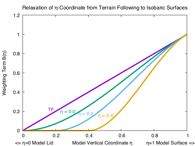
Fig. 5.1 The transition of the h coordinate surfaces from terrain following (TF) to isobaric is a function of the critical value of h at which the user requests that an isobaric surface be achieved. The fundamental property of the TF vs. the HVC system is seen when tracing a horizontal line from any value on the “Weighting Term B(h)” axis. The degree of model coordinate  “flatness”, for example, is the same in the TF system at h = 0.2 as in the HVC system for h_C = 0.4 when the approximate value of h = 0.6.

 

 

The depiction of the vertical location of an h surface for an isobaric coordinate (figure 5.2a), a terrain following coordinate (figure 5.2b), and a hybrid coordinate (figure 5.2c) is given with a simple 2d cross section. The depth of the atmosphere (m) and pressure are shown.

 

 

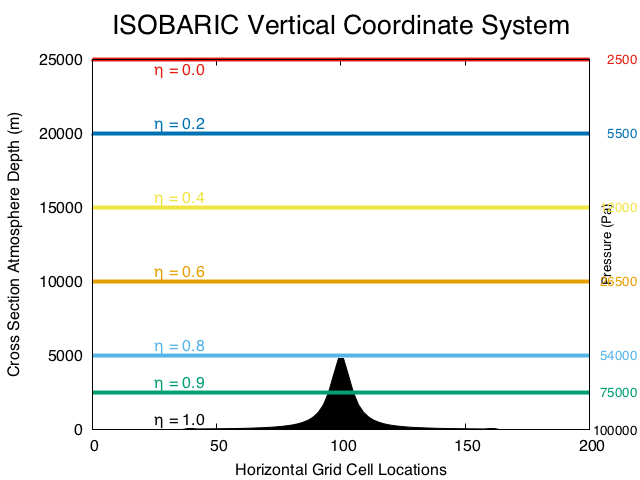
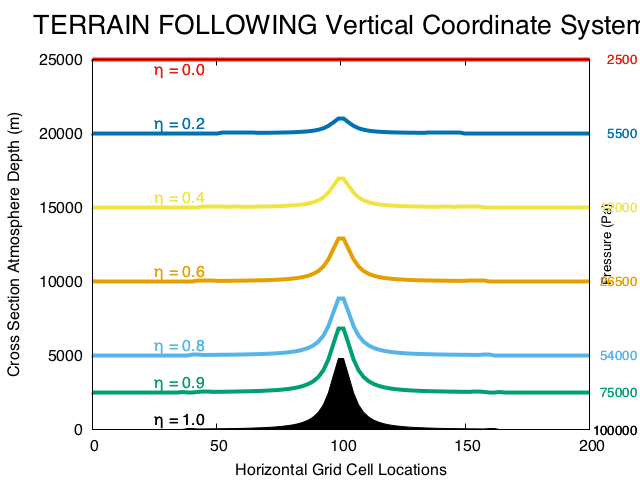
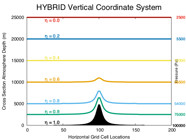
Fig. 5.2 Three cross section plots show the vertical location of the h surfaces for a given model lid (25 km is approximately 25 hPa) and for a given h_C = 0.2.

 

If you wish to revert to the TF coordinate option, you will need to set hybrid_opt=0 in the &dynamics section of the namelist. The real.exe and wrf.exe programs must both run with the same hybrid_opt value.

 

Use care when sending the HVC data to post-processors, which must know the new definition of dry pressure. It is advised that either hydrostatic pressure (P_HYD) or total pressure (PB + P) be used for diagnostics and for vertical interpolations.

 

u. Use of Multiple Lateral Condition Files

 

To speed up pre-processing of lateral boundary conditions in real-time scenarios, an option to create multiple lateral condition files was previously done through a compile option (adding -D_MULTI_BDY_FILES_ in ARCH_LOCAL in the configure.wrf file). This allows a boundary condition file to be created as soon as the surrounding time periods become available, allowing the model to start the simulation sooner. Since V4.2, this can be achieved through a runtime option, by adding the following to namelist.input.

     &time_control

     bdy_inname      = "wrfbdy_d<domain>_<date>"

and

     &bdy_control

     multi_bdy_files = .true.

 

Output files are (using a 6-hourly data interval)

     wrfbdy_d01_2000-01-24_12:00:00

     wrfbdy_d01_2000-01-24_18:00:00

     wrfbdy_d01_2000-01-25_00:00:00

     wrfbdy_d01_2000-01-25_06:00:00

 

v. Use of MAD-WRF

 

The MAD-WRF model is designed to improve the cloud analysis and solar irradiance short-range forecast.

 

There are two options to run MAD-WRF:

            1. madwrf_opt = 1: The initial hydrometeors are advected and diffused with the

                                            model dynamics without accounting for any microphysical

                                            processes. Users should set mp_physics = 96 and

                                            use_mp_re = 0 in the physics block of namelist.input.

 

            2. madwrf_opt = 2: There is a set of hydrometeor tracers that are advected and

                                            diffused with the model dynamics. At initial time the tracers

                                            are equal to the standard hydrometeors. During the simulation

                                            the standard hydrometeors are nudged toward the tracers.                                                    The namelist variable madwrf_dt_nudge sets the temporal

                                            period for hydrometeor nudging [min]. Namelist

                                            madwrf_dt_relax sets the relaxation time for hydrometeor

                                            nudging [s].

 

 

MAD-WRF has an option to enhance cloud initialization. To turn on (off) cloud initialization, set the namelist variable madwrf_cldinit=1 (0).

 

By default the model enhances cloud analysis based on the analyzed relative humidity.

Users can enhance cloud initialization by providing additional variables to metgrid via the WPS intermediate format:

 

            1. Cloud mask (CLDMASK variable):

                        Remove clouds if clear (cldmask = 0)

 

            2. Cloud mask (CLDMASK variable) + brightness temperature (BRTEMP

            variable) sensitive to hydrometeor content (e.g. GOES-R channel 13):

                        Remove clouds if clear (cldmask = 0)

                        Reduce / extend cloud top heights to match observations

                        Add clouds over clear sky regions (cldmask = 1)

 

            3. Cloud top height (CLDTOPZ variable) with 0 values over clear sky regions:

                         Remove clouds if clear (cldmask = 0)

                         Reduce / extend cloud top heights to match observations

                        Add clouds over clear sky regions (cldmask = 1)

 

            4. Either 2 or 3 + the cloud base height (CLDBASEZ variable):

                        Remove clouds if clear (cldmask = 0)

                        Reduce / extend cloud top / base heights to match observations

 

            *Missing values in any of these variables should be set to -999.9

Examples of namelists for various applications

A few physics option sets (plus model top and the number of vertical levels) are provided here for reference. They may provide a good starting point for testing the model in your application. Note that other factors will affect the outcome; for example, the domain setup, distributions of vertical model levels, and input data.

a. 1 – 4 km grid distances, convection-permitting runs for a 1- 3 day run (as was used for the NCAR spring real-time convection forecast over the US in 2013 and 3 km ensemble in 2015 – 2017, and this is the ‘CONUS’ physics suite without the cumulus scheme):

mp_physics                          = 8,
ra_lw_physics                       = 4,
ra_sw_physics                       = 4,
radt                                = 10,
sf_sfclay_physics                   = 2,
sf_surface_physics                  = 2,
bl_pbl_physics                      = 2,
bldt                                = 0,
cu_physics                          = 0,

ptop_requested                      = 5000,
e_vert                              = 40,

b. 10 – 20 km grid distances, 1- 3 day runs (e.g., previous NCAR daily real-time runs over the US):

mp_physics                          = 8,
ra_lw_physics                       = 4,
ra_sw_physics                       = 4,
radt                                = 15,
sf_sfclay_physics                   = 1,
sf_surface_physics                  = 2,
bl_pbl_physics                      = 1,
bldt                                = 0,
cu_physics                          = 3,
cudt                                = 0,

ptop_requested                      = 5000,
e_vert                              = 39,

c. Cold region 10 – 30 km grid sizes (e.g. used in NCAR’s Antarctic Mesoscale Prediction System):

mp_physics                          = 4,
ra_lw_physics                       = 4,
ra_sw_physics                       = 2,
radt                                = 15,
sf_sfclay_physics                   = 2,
sf_surface_physics                  = 2,
bl_pbl_physics                      = 2,
bldt                                = 0,
cu_physics                          = 1,
cudt                                = 5,
fractional_seaice                   = 1,
seaice_threshold                    = 0.0,

ptop_requested                      = 1000,
e_vert                              = 44,

d. Hurricane applications (e.g. 36, 12, and 4 km nesting used by NCAR’s real-time hurricane runs in 2012):

mp_physics                          = 6,
ra_lw_physics                       = 4,
ra_sw_physics                       = 4,
radt                                = 10,
sf_sfclay_physics                   = 1,
sf_surface_physics                  = 2,
bl_pbl_physics                      = 1,
bldt                                = 0,
cu_physics                          = 6, (only on 36/12 km grid)
cudt                                = 0,
isftcflx                            = 2,

ptop_requested                      = 2000,
e_vert                              = 36,

e. Regional climate case at 10 – 30 km grid sizes (e.g. used in NCAR’s regional climate runs):

mp_physics                          = 6,
ra_lw_physics                       = 3,
ra_sw_physics                       = 3,
radt                                = 30,
sf_sfclay_physics                   = 1,
sf_surface_physics                  = 2,
bl_pbl_physics                      = 1,
bldt                                = 0,
cu_physics                          = 1,
cudt                                = 5,
sst_update                          = 1,
tmn_update                          = 1,
sst_skin                            = 1,
bucket_mm                           = 100.0,
bucket_J                            = 1.e9,
ptop_requested                      = 1000,
e_vert                              = 51,

spec_bdy_width                      = 10,
spec_zone                           = 1,
relax_zone                          = 9,
spec_exp                            = 0.33,

 

Check Output

Once a model run completes, it is advised to quickly check a few things.

If you built the model with distributed memory (dmpar), you should have an rsl.out.* and rsl.error.* file for each processor. Type ‘tail rsl.out.0000’ to see if you get ‘SUCCESS COMPLETE WRF,’ which indicates the model ran successfully.

Namelist options are written to a separate file, “namelist.output.”

Check the output times written to the wrfout* file by using the netCDF command:

  ncdump –v Times wrfout_d01_yyyy-mm-dd_hh:00:00

Take a look at either the rsl.out.0000 file (or other standard-out files), which logs the times taken to compute for one model time step, and to write one history and restart output file:

Timing for main: time 2006-01-21_23:55:00 on domain  2:    4.91110 elapsed seconds.

Timing for main: time 2006-01-21_23:56:00 on domain  2:    4.73350 elapsed seconds.

Timing for main: time 2006-01-21_23:57:00 on domain  2:    4.72360 elapsed seconds.

Timing for main: time 2006-01-21_23:57:00 on domain  1:   19.55880 elapsed seconds.

and

Timing for Writing wrfout_d02_2006-01-22_00:00:00 for domain 2: 1.17970 elapsed seconds.

Timing for main: time 2006-01-22_00:00:00 on domain 1: 27.66230 elapsed seconds.

Timing for Writing wrfout_d01_2006-01-22_00:00:00 for domain 1: 0.60250 elapsed seconds.

 

Trouble Shooting

-       If the model aborts very quickly, it is likely that either the computer memory is not large enough to run the specific configuration, or the input data have some serious problems. For the first issue, type ‘unlimit’ or ‘ulimit -s unlimited’ (prior to configuring and compiling) to see if more memory and/or stack size can be obtained.

-       For OpenMP (smpar-compiled code), the stack size needs to be set large, but not unlimited. Unlimited stack size may crash the computer.

-       To check if the input data are the problem, use ncview or another netCDF file browser to check fields in the wrfinput files.

-       Another frequent error seen is ‘ERRORS while reading one or more namelists from namelist.input’. This is an error message from the model complaining about errors and typos in the namelist.input file. Above the error message, the model tries to determine where the namelist has problems. Check and modify the line(s) mentioned. Edit the namelist.input file with caution. If unsure, always start with an available default template.

-       If the model did not run to completion, one possibility is the model may have become numerically unstable, meaning the time step used for advancing the model in time is too large for a stable solution. Even if one observes the standard rule for setting the model time step (to be no more than 6*DX in km in physical space), other configurations of the model domain may affect the outcome. For example, if the model layers are too thin, or if you use a very large domain and the corners of the domain have a large map-scale factor that reduces the equivalent earth distance to be much smaller than the model grid size. Check the rsl.error.* files for cfl errors.

 

grep cfl rsl.error.* or grep cfl wrf.out

you may see something like:

5 points exceeded cfl=2 in domain            1 at time   4.200000 

  MAX AT i,j,k:          123          48          3 cfl,w,d(eta)= 4.165821

21 points exceeded cfl=2 in domain            1 at time   4.200000 

  MAX AT i,j,k:          123          49          4 cfl,w,d(eta)= 10.66290
 
When this happens, consider using the namelist option w_damping, and/or reducing the time step.

 

Physics and Dynamics Options

Physics Options

WRF offers multiple physics options that can be combined in any way. The options typically range from simple and efficient, to sophisticated and more computationally costly, and from newly developed schemes, to well-tried schemes such as those in current operational models.

The choices vary with each major WRF release, but here we will outline those available in WRF Version 4.

1. Microphysics (mp_physics)

a. Kessler scheme: A warm-rain (i.e. no ice) scheme used commonly in idealized cloud modeling studies (mp_physics = 1).

b. Purdue Lin scheme: A sophisticated scheme that has ice, snow and graupel processes, suitable for real-data high-resolution simulations (2).

c. WRF Single-Moment 3-class scheme: A simple, efficient scheme with ice and snow processes suitable for mesoscale grid sizes (3).

d. WRF Single-Moment 5-class scheme: A slightly more sophisticated version of (c) that allows for mixed-phase processes and super-cooled water (4).

e. Ferrier Eta microphysics: The operational microphysics in NCEP models. A simple efficient scheme with diagnostic mixed-phase processes. For fine resolutions (< 5km) use option (5) and for coarse resolutions use option (95).

f. WRF Single-Moment 6-class scheme: A scheme with ice, snow and graupel processes suitable for high-resolution simulations (6).

g. Goddard 4-ice microphysics scheme (7) predicts hail and graupel separately, provides effective radii for radiation. Replaced older Goddard scheme in V4.1.

h.  Thompson et al. scheme: A scheme with ice, snow and graupel processes suitable for high-resolution simulations (8).

i. Milbrandt-Yau Double-Moment 7-class scheme (9). This scheme includes separate

categories for hail and graupel with double-moment cloud, rain, ice, snow, graupel and hail.

j. Morrison double-moment scheme (10). Double-moment ice, snow, rain and graupel for cloud-resolving simulations.

k. CAM V5.1 2-moment 5-class scheme.

l. Stony Brook University (Y. Lin) scheme (13). This is a 5-class scheme with riming intensity predicted to account for mixed-phase processes.

m. WRF Double-Moment 5-class scheme (14). This scheme has double-moment rain. Cloud and CCN for warm processes, but is otherwise like WSM5.

n. WRF Double-Moment 6-class scheme (16). This scheme has double-moment rain. Cloud and CCN for warm processes, but is otherwise like WSM6.

o. NSSL 2-moment scheme (17, 18, 19, 21, 22). Option (17) is a two-moment scheme for cloud droplets, rain drops, ice crystals, snow, graupel, and hail. It also predicts average graupel particle density, which allows graupel to span the range from frozen drops to low-density graupel. Option (18) is similar, but also predicts cloud condensation nuclei (CCN) concentration (intended for idealized simulations). The scheme is intended for cloud-resolving simulations (dx <= 2km) in research applications. Option (19) is a single-moment version of the NSSL scheme, and option (21) is similar to Gilmore et al. (2004). Option (22) is the two moment scheme (option 17) without hail.

p. WSM7 (24). As WSM6, but adding a hail category. New in V4.1.

q. WDM7 (26). As WDM6, but adding a hail category. New in V4.1.

r. Thompson aerosol-aware (28). This scheme considers water- and ice-friendly aerosols. A climatology dataset may be used to specify initial and boundary conditions for the aerosol variables (Thompson and Eidhammer, 2014, JAS.) This includes a surface dust scheme.

s. HUJI (Hebrew University of Jerusalem, Israel) spectral bin microphysics, full (32) and ‘fast’ (30) versions are available.

t. Morrison double-moment scheme with CESM aerosol (40): must be used together with MSKF cumulus scheme.

u. P3 (Morrison and Milbrandt) (50, 51, 52, 53): Predicted Particle Property scheme. This has one ice category that represents a combination of ice, snow and graupel, and also carries prognostic arrays for rimed ice mass and rimed ice volume. Double moment rain and ice (50). P3-nc (51): As in 50, but adds supersaturation dependent activation and double-moment cloud water. P3-2ice (52): As in P3-nc but with two arrays for ice. P3-3moment: As in P3-nc (51), but with 3-moment ice.

v. Jensen ISHMAEL (55): Scheme that predicts particle shapes and habits in ice crystal growth. New in V4.1.

w. National Taiwan University (NTU) (56): double-moments for the liquid phase, and triple-moments for the ice phase, together with consideration for ice crystal shape and density variations. Supersaturation is resolved so that condensation nuclei (CN) activation is explicitly calculated; CN’s mass in droplets is tracked to account for aerosol recycling. (Tsai and Chen, 2020, JAS)

 

2.1 Longwave Radiation (ra_lw_physics)

a. RRTM scheme (ra_lw_physics = 1): Rapid Radiative Transfer Model. An accurate scheme using look-up tables for efficiency. Accounts for multiple bands, and microphysics species. For trace gases, the volume-mixing ratio values for
CO₂=379e-6, N₂O=319e-9 and CH4=1774e-9. See section 2.3 for time-varying option.

b. CAM scheme (3): from the CAM 3 climate model used in CCSM. Allows for aerosols and trace gases. It uses yearly CO₂, and constant N₂O (311e-9) and CH₄ (1714e-9). See section 2.3 for the time-varying option.

c. RRTMG scheme (4): A newer version of RRTM. It includes the MCICA method of random cloud overlap. For major trace gases, CO₂=379e-6 (valid for 2005), N₂O=319e-9, CH₄=1774e-9. See section 2.3 for the time-varying option. Since V4.2, the CO₂ value is replaced by a function of the year: CO2(ppm) = 280 + 90 exp (0.02*(year-2000)), which has about 4% of error for 1920s and 1960s, and about 1 % after year 2000 when compared to observed values.

d. Goddard scheme (5). Efficient, multiple bands, ozone from simple climatology. Designed to run with Goddard microphysics particle radius information. Updated in V4.1.

e. Fu-Liou-Gu scheme (7). multiple bands, cloud and cloud fraction effects, ozone profile from climatology and tracer gases. CO₂=345e-6.

f. RRTMG-K scheme (14): A version of RRTMG scheme improved by Baek (2017), A revised radiation package of G-packed McICA and two-stream approximation: Performance evaluation in a global weather forecasting model, J. Adv. Model. Earth Syst., 9, doi:10.1002/2017MS000994).    

g. RRTMG-fast scheme (24): A fast version of the RRTMG scheme.  

h. GFDL scheme (99): Eta operational radiation scheme. An older multi-band scheme with carbon dioxide, ozone and microphysics effects.

 

2.2 Shortwave Radiation (ra_sw_physics)

a. Dudhia scheme: Simple downward integration allowing efficiently for clouds and clear-sky absorption and scattering (ra_sw_physics = 1).

b. Goddard shortwave: Two-stream multi-band scheme with ozone from climatology and cloud effects (2).

c. CAM scheme: from the CAM 3 climate model used in CCSM. Allows for aerosols and trace gases (3).

d. RRTMG shortwave. A new shortwave scheme with the MCICA method of random cloud overlap (4). For major trace gases, CO₂=379e-6 (valid for 2005), N₂O=319e-9, CH₄=1774e-9. See section 2.3 for the time-varying option. Since V4.2, the CO₂ value is replaced by a function of the year: CO2(ppm) = 280 + 90 exp (0.02*(year-2000)), which has about 4% of error for 1920s and 1960s, and about 1 % after year 2000 when compared to observed values.

e Goddard scheme (5). Efficient, multiple bands, ozone from simple climatology. Designed to run with Goddard microphysics particle radius information. Updated in V4.1.

f. Fu-Liou-Gu scheme (7). multiple bands, cloud and cloud fraction effects, ozone profile from climatology, can allow for aerosols.

g. RRTMG-K (14): A version of RRTMG scheme improved by Baek (2017).

h. RRTMG-fast shortwave. A fast version of RRTMG.

i. Held-Suarez relaxation. A temperature relaxation scheme designed for idealized tests only (31).

j. GFDL shortwave: Eta operational scheme. Two-stream multi-band scheme with ozone from climatology and cloud effects (99).

 

Related options:

- slope_rad = 1: Slope and shading effects. The option modifies surface solar radiation flux according to terrain slope. topo_shading = 1 allows for shadowing of neighboring grid cells. Use only with high-resolution runs with grid size less than a few kilometers.

- swrad_scat: scattering turning parameter for ra_sw_physics = 1. Default value is 1, which is equivalent to 1.e-5 m²/kg. When the value is greater than 1, scattering is increased.

- ra_sw_eclipse = 1: Eclipse effect on shotwave radiation. Works for RRTMG (4), Goddard (5), old Goddard (2) and Duhhia (1) shortwave radiation options. The eclipse data from 1950 – 2050 is provided in run/eclipse_besselian_elements.dat.

- swint_opt = 1: Interpolation of short-wave radiation based on the updated solar zenith angle between shortwave calls.

 

- swint_opt = 2 activates the Fast All-sky Radiation Model for Solar applications (FARMS). FARMS is a fast radiative transfer model that allows simulations of broadband solar radiation every model time step. The model uses lookup tables of cloud transmittances and reflectances by varying cloud optical thicknesses, cloud particle sizes, and solar zenith angles. A more detailed description is provided in Xie et al. (2016).

2.3 Input to radiation options

a. CAM Green House Gases: Provides yearly green house gases from 1765 to 2500. This option is activated by compiling WRF with the macro –DCLWRFGHG added in configure.wrf. Once compiled, CAM, RRTM and RRTMG long-wave schemes will see these gases. Five scenario files are available: from IPCC AR5: CAMtr_volume_mixing_ratio .RCP4.5, CAMtr_volume_mixing_ratio.RCP6, and CAMtr_volume_mixing_ratio.RCP8.5; from IPCC AR4: CAMtr_volume_mixing_ratio.A1B, and CAMtr_volume_mixing_ratio.A2. The default points to the RCP8.5 file.

b. Climatological ozone and aerosol data for RRTMG: The ozone data are adapted from CAM radiation (ra_*_physics=3), and have latitudinal (2.82 degrees), height, and temporal (monthly) variation, as opposed to the default ozone used in the scheme that only varies with height. This is activated by the namelist option o3input=2, which is the default option. The aerosol data are based on Tegen et al. (1997), which has 6 types: organic carbon, black carbon, sulfate, sea salt, dust and stratospheric aerosol (volcanic ash, which is zero). The data also have spatial (5 degrees in longitude and 4 degrees in latitudes) and temporal (monthly) variations. The option is activated by the namelist option aer_opt=1.

c. Aerosol input for RRTMG and Goddard radiation options (aer_opt=2). Either AOD or AOD plus Angstrom exponent, single scattering albedo, and cloud asymmetry parameter can be provided via constant values from the namelist or 2D input fields via auxiliary input stream 15. Aerosol type can also be set.

d. Aerosol input for RRTMG radiation scheme from climatological water- and ice-friendly aerosols (aer_opt=3). It works with Thompson microphysics option 28.

e. Effective cloud water, ice and snow radii from Thompson, WSM, WDM and NSSL, and P3 microphysics schemes are used in RRTMG.

 

2.4 Cloud fraction option

icloud: = 1, use Xu-Randall method; = 2, use threshold method which gives either 0 or 1 cloud fraction; = 3, use a RH-based method that follows Sundqvist et al. (1989). The threshold of RH depends on grid sizes.

 

 

3.1 Surface Layer (sf_sfclay_physics)

a. Revised MM5 surface layer scheme (1): Remove limits and use updated stability functions (Jimenez et al. MWR 2012). Thermal and moisture roughness lengths (or exchange coefficients for heat and moisture) over the ocean use the COARE 3 formula (Fairall et al. 2003).

b.  Eta similarity: Used in Eta model. Based on Monin-Obukhov with Zilitinkevich thermal roughness length and standard similarity functions from look-up tables (2).

c. QNSE surface layer. Quasi-Normal Scale Elimination PBL scheme’s surface layer option (4).

d. MYNN surface layer. Nakanishi and Niino PBL’s surface layer scheme (5).

e. Pleim-Xiu surface layer. (7).

f. TEMF surface layer. Total Energy – Mass Flux surface layer scheme (10).

g. MM5 similarity: Based on Monin-Obukhov with Carslon-Boland viscous sub-layer and standard similarity functions from look-up tables (sf_sfclay_physics = 91). The thermal and moisture roughness lengths (or exchange coefficients for heat and moisture) over ocean use the COARE 3 formula (Fairall et al. 2003).

h. Other: iz0tlnd = 1 (works with sf_sfclay_physics = 1, 91, and 5), Chen-Zhang thermal roughness length over land, which depends on vegetation height, 0 = original thermal roughness length in each sfclay option.

 

3.2 Land Surface (sf_surface_physics)

a. (1) 5-layer thermal diffusion: Soil temperature only scheme, using five layers.

b. (2) Noah Land Surface Model: Unified NCEP/NCAR/AFWA scheme with soil temperature and moisture in four layers, fractional snow cover and frozen soil physics.

- A sub-tiling option can be activated by namelist sf_surface_mosaic = 1, and the number of tiles in a grid box is defined by namelist mosaic_cat, with a default value of 3.

      c. (3) RUC Land Surface Model: This model uses a layer approach to the solution of energy and moisture budgets. Atmospheric and soil fluxes are computed in the middle of the first atmospheric layer and the top soil layer, respectively, and these fluxes modify the heat and moisture storage in the layer spanning the ground surface. The RUC LSM uses 9 soil levels with higher resolution near the interface with the atmosphere. (NOTE: if initialized from the model with low resolution near the surface, like the Noah LSM, the top levels could be too moist causing moist/cold biases in the model forecast. Solution: cycle soil moisture and let it spin-up for several days to fit the vertical structure of RUC LSM).

 

The prognostic variable for soil moisture is volumetric soil moisture content, minus the residual soil moisture tied to soil particles, and therefore not participating in moisture transport. The RUC LSM takes into account freezing and thawing processes in the soil. It is able to use explicit mixed-phase precipitation provided by cloud microphysics schemes. It uses a simple treatment of sea ice, which solves heat diffusion in sea ice and allows evolving snow cover on top of sea ice. In the warm season, RUC LSM corrects soil moisture in cropland areas to compensate for irrigation in these regions.

 

Snow accumulated on top of soil can have up to two layers, depending on snow depth (ref S16). When the snow layer is very thin, it is combined with the top soil layer to avoid excessive radiative cooling at night. The grid cell can be partially covered with snow, when snow water equivalent is below a threshold value of 3 cm. When this condition occurs, surface parameters, such as roughness length and albedo, are computed as a weighted average of snow-covered and snow-free areas. The energy budget utilizes an iterative snow melting algorithm. Melted water can partially refreeze and remain within the snow layer, and the rest of it percolates through the snow pack, infiltrates into soil and forms surface runoff. Snow density evolves as a function of snow temperature, snow depth and compaction parameters. Snow albedo is initialized from the maximum snow albedo for the given vegetation type, but it can also be modified, depending on snow temperature and snow fraction. To obtain a better representation of snow accumulated on the ground, the RUC LSM has introduced estimation of frozen precipitation density.

 

The most recent modifications to RUC LSM include refinements to the interception of liquid or frozen precipitation by the canopy, and also the “mosaic” approach for patchy snow with a separate treatment of energy and moisture budgets for snow-covered and snow-free portions of the grid cell, and aggregation of the separate solutions at the end of time step.

 

The datasets needed to initialize RUC LSM include: 

1.   High-resolution dataset for soil and land-use types; 

2.   Climatological albedo for snow-free areas;

3.   Spatial distribution of maximum surface albedo in the presence of snow cover;

4.   Fraction of vegetation types in the grid cell to take into account sub-grid-scale             heterogeneity in computation of surface parameters;

5.   Fraction of soil types within the grid cell;

6.   Climatological greenness fraction;

7.   Climatological leaf area index;

8.   Climatological mean temperature at the bottom of soil domain;

9.   Real-time sea-ice concentration;

10. Real-time snow cover to correct cycled in RAP and HRRR snow fields.

 

Recommended namelist options:

   sf_surface_physics  = 3

   num_soil_layers     = 9,

   usemonalb           = .true.,

   rdlai2d             = .true.,

   mosaic_lu           = 1

   mosaic_soil         = 1

 

References:

Smirnova et al (2016, Mon. Wea. Rev., S16);

RAP and HRRR that use RUC LSM as their land component: https://rapidrefresh.noaa.gov/RAP and https://rapidrefresh.noaa.gov/hrrr/HRRR.

 

(from Tanya Smirnova, GSD/NOAA)

 

d. (4) Noah-MP (multi-physics) Land Surface Model: uses multiple options for key land-atmosphere interaction processes. Noah-MP contains a separate vegetation canopy defined by a canopy top and bottom with leaf physical and radiometric properties used in a two-stream canopy radiation transfer scheme that includes shading effects. Noah-MP contains a multi-layer snow pack with liquid water storage and melt/refreeze capability and a snow-interception model describing loading/unloading, melt/refreeze, and sublimation of the canopy-intercepted snow. Multiple options are available for surface water infiltration and runoff, and groundwater transfer and storage including water table depth to an unconfined aquifer. Horizontal and vertical vegetation density can be prescribed or predicted using prognostic photosynthesis and dynamic vegetation models that allocate carbon to vegetation (leaf, stem, wood and root) and soil carbon pools (fast and slow). (Niu et al. 2011)

e.  (5) CLM4 (Community Land Model Version 4, Oleson et al. 2010; Lawrence et al. 2010): CLM4 contains sophisticated treatment of biogeophysics, hydrology, biogeochemistry, and dynamic vegetation. In CLM4, the land surface in each model grid cell is characterized into five primary sub-grid land cover types (glacier, lake, wetland, urban, and vegetated). The vegetated sub-grid consists of up to 4 plant functional types (PFTs) that differ in physiology and structure. The WRF input land cover types are translated into the CLM4 PFTs through a look-up table. The CLM4 vertical structure includes a single-layer vegetation canopy, a five-layer snowpack, and a ten-layer soil column. An earlier version of CLM has been quantitatively evaluated within WRF in Jin and Wen (2012; JGR-Atmosphere), Lu and Kueppers (2012; JGR-Atmosphere), and Subin et al. (2011; Earth Interactions) (from Jin).

f. (7) Pleim-Xiu Land Surface Model. For a more detailed description of the PX LSM, including pros/cons, best practices, and recent improvements, see http://www2.mmm.ucar.edu/wrf/users/docs/PX-ACM.pdf

Two-layer scheme with vegetation and sub-grid tiling. The Pleim-Xiu land surface model (PX LSM; Pleim and Xiu 1995; Xiu and Pleim 2001) was developed and improved over the years to provide realistic ground temperature, soil moisture, and surface sensible and latent heat fluxes in mesoscale meteorological models. The PX LSM is based on the ISBA model (Noilhan and Planton 1989), and includes a 2-layer force-restore soil temperature and moisture model.  the top layer is taken to be 1 cm thick, and the lower layer is 99 cm. Grid aggregate vegetation and soil parameters are derived from fractional coverage of land use categories and soil texture types. There are two indirect nudging schemes that correct biases in 2-m air temperature and moisture by dynamic adjustment of soil moisture (Pleim and Xiu, 2003) and deep soil temperature (Pleim and Gilliam, 2009).

Users should recognize that the PX LSM was primarily developed for retrospective simulation, where surface-based observations are available to inform the indirect soil nudging. While soil nudging can be disabled using the FDDA namelist.input setting pxlsm_soil_nudge, little testing has been done in this mode, although some users have reported reasonable results. Gilliam and Pleim (2010) discuss the implementation in the WRF model and provide typical configurations for retrospective applications. If soil nudging is activated, modelers must use the Obsgrid objective re-analysis utility (https://www2.mmm.ucar.edu/wrf/users/docs/user_guide_v4/v4.2/users_guide_chap7.html) to produce a surface nudging file with the naming convention "wrfsfdda_d0*."  Obsgrid takes WPS "met_em*" files and LittleR observation files and produces the "wrfsfdda_d0*" file.  The PX LSM uses 2-m temperature and mixing ratio re-analyses from this file for the deep soil moisture and temperature nudging.  If modelers want to test PX LSM in forecast mode with soil nudging activated, forecasted 2-m temperature and mixing ratio can be used with empty observation files to produce the "wrfsfdda_d0*" files, using Obsgrid, but results are tied to the governing forecast model.

 f. (8) SSiB Land Surface Model: This is the third generation of the Simplified Simple Biosphere Model (Xue et al. 1991; Sun and Xue, 2001). SSiB is developed for land/atmosphere interaction studies in the climate model. The aerodynamic resistance values in SSiB are determined in terms of vegetation properties, ground conditions and bulk Richardson number according to the modified Monin–Obukhov similarity theory. SSiB-3 includes three snow layers to realistically simulate snow processes, including destructive metamorphism, densification process due to snow load, and snow melting, which substantially enhances the model’s ability for the cold season study. To use this option, ra_lw_physics and ra_sw_physics should be set to either 1, 3, or 4. The second full model level should be set to no larger than 0.982 so that the height of that level is higher than vegetation height.

h. Fractional sea-ice (fractional_seaice=1). Treat sea-ice as a fractional field. Requires fractional sea-ice as input data. Data sources may include those from GFS or the National Snow and Ice Data Center (https://nsidc.org/). Use XICE for the Vtable entry instead of SEAICE. This option works with sf_sfclay_physics = 1, 2, 5, and 7, and sf_surface_physics = 2, 3, and 7.

 

 

3.3 Urban Surface (sf_urban_physics – replacing old switch ucmcall)

Urban physics options work with the Noah LSM, and with NoahMP. Beginning in V4.3, code is updated to include a capability to use local climate zones, which is incorporated for all three urban applications (additional information can be found here).

a. Urban canopy model (1): 3-category UCM option with surface effects for roofs, walls, and streets. Includes a green roof option.

b. BEP (2). Building Environment Parameterization: Multi-layer urban canopy model that allows for buildings higher than the lowest model levels. Works with Noah and NoahMP LSM, and Boulac, MYJ PBL and YSU options.

c. BEM (3). Building Energy Model. Adds to BEP, building energy budget with heating and cooling systems. Works with same options as BEP.

 

3.4 Lake Physics (sf_lake_physics)

a. CLM 4.5 lake model (1). The lake scheme was obtained from the Community Land Model version 4.5 (Oleson et al. 2013) with some modifications by Gu et al. (2013). It is a one-dimensional mass and energy balance scheme with 20-25 model layers, including up to 5 snow layers on the lake ice, 10 water layers, and 10 soil layers on the lake bottom. The lake scheme is used with actual lake points and lake depth derived from the WPS, and can also be used with user-defined lake points and lake depth in WRF (lake_min_elev and lakedepth_default). The lake scheme is independent of a land surface scheme and therefore can be used with any land surface scheme embedded in WRF. The lake scheme developments and evaluations were included in Subin et al. (2012) and Gu et al. (2013) (Subin et al. 2012: Improved lake model for climate simulations, J. Adv. Model. Earth Syst., 4, M02001. DOI:10.1029/2011MS000072; Gu et al. 2013: Calibration and validation of lake surface temperature simulations with the coupled WRF-Lake model. Climatic Change, 1-13, 10.1007/s10584-013-0978-y). 

 

4. Planetary Boundary layer (bl_pbl_physics)

a. Yonsei University scheme: Non-local-K scheme with explicit entrainment layer and parabolic K profile in unstable mixed layer (bl_pbl_physics = 1).

- topo_wind: = 1: Topographic correction for surface winds to represent extra drag from sub-grid topography and enhanced flow at hill tops (Jimenez and Dudhia, JAMC 2012). Works with YSU PBL only. (topo_wind= 2): a simpler terrain variance-related correction.

- ysu_topdown_pblmix: = 1: option for top-down mixing driven by radiative cooling.

b. Mellor-Yamada-Janjic scheme: Eta operational scheme. One-dimensional prognostic turbulent kinetic energy scheme with local vertical mixing (2).

c. Quasi-Normal Scale Elimination PBL (4). A TKE-prediction option that uses a new theory for stably stratified regions. Daytime part uses eddy diffusivity mass-flux method with shallow convection (mfshconv = 1).

d. Mellor-Yamada Nakanishi and Niino Level 2.5 PBL (5). Predicts sub-grid TKE terms.

- icloud_bl: = 1, option to couple subgrid-scale clouds from MYNN to radiation;
- bl_mynn_cloudpdf: = 1, Kuwano et al (2010); = 2, Chaboureau and Bechtold (2002, JAS, with mods, default);
- bl_mynn_cloudmix: = 1, mixing cloud water and ice (qnc and qni are mixed when scalar_pblmix = 1);
- bl_mynn_edmf = 1, activate mass-flux in MYNN;
- bl_mynn_mixlength = 2: 1 is from RAP/HRRR, 2 is from blending.

e. Mellor-Yamada Nakanishi and Niino Level 3 PBL (6). Predicts TKE and other second-moment terms.

f. ACM2 PBL: Asymmetric Convective Model with non-local upward mixing and local downward mixing (7).

g. BouLac PBL (8): Bougeault-Lacarrère PBL. A TKE-prediction option. Designed for use with BEP urban model.

h. UW (Bretherton and Park) scheme (9). TKE scheme from CESM climate model.

i. Total Energy - Mass Flux (TEMF) scheme (10). Sub-grid total energy prognostic variable, plus mass-flux type shallow convection.

j. Shin-Hong scheme (11): Include scale dependency for vertical transport in convective PBL. Vertical mixing in the stable PBL and free atmosphere follows YSU. This scheme also has diagnosed TKE and mixing length output.

k. Grenier-Bretherton-McCaa scheme (12): This is a TKE scheme. Tested in cloud-topped PBL cases.

l. MRF scheme: Older version of (a) with implicit treatment of entrainment layer as part of non-local-K mixed layer (99).

m. LES PBL: A large-eddy-simulation (LES) boundary layer is available. For this, bl_pbl_physic = 0, isfflx = 1, and sf_sfclay_physics and sf_surface_physics are selected. This uses diffusion for vertical mixing and must use diff_opt = 2, and km_opt = 2 or 3, see below. Alternative idealized ways of running the LESPBL are chosen with isfflx = 0 or 2.

n. SMS-3DTKE: This is a 3D TKE subgrid mixing scheme that is self-adaptive to the grid size between the large-eddy simulation (LES) and mesoscale limits. It can be activated by setting bl_pbl_physic = 0, km_opt = 5, diff_opt=2 and can only be used with sf_sfclay_physics = 1, 5, 91. New in Version 4.2.

o. TKE (E)-TKE dissipation rate (epsilon) scheme (16), EEPS: This scheme predicts TKE as well as TKE dissipation rate. It also advects both TKE and the dissipation rate. It works with surface layer physics option 1, 91, and 5.

5. Cumulus Parameterization (cu_physics)

a. Kain-Fritsch scheme: Deep and shallow convection sub-grid scheme using a mass flux approach with downdrafts and CAPE removal time scale (cu_physics = 1).

-  kfeta_trigger = 1 – default trigger; = 2 – moisture-advection modulated trigger function [based on Ma and Tan (2009, Atmospheric Research)]. May improve results in subtropical regions when large-scale forcing is weak.

- cu_rad_feedback = true – allow sub-grid cloud fraction interaction with radiation. (Alapaty et al. 2012, Geophysical Research Letters)

b. Betts-Miller-Janjic scheme. Operational Eta scheme. Column moist adjustment scheme relaxing towards a well-mixed profile (2).

c. Grell-Freitas (GF) scheme (3): An improved GD scheme that tries to smooth the transition to cloud-resolving scales, as proposed by Arakawa et al. (2004).

d. Simplified Arakawa-Schubert (SAS) (4). Simple mass-flux scheme with quasi-equilibrium closure with shallow mixing scheme (and momentum transport in NMM only).

e. Grell 3D is an improved version of the GD scheme that may also be used on high resolution (in addition to coarser resolutions) if subsidence spreading (option cugd_avedx) is turned on (5).

f. Tiedtke scheme (U. of Hawaii version) (6). Mass-flux type scheme with CAPE-removal time scale, shallow component and momentum transport.

g. Zhang-McFarlane scheme (7). Mass-flux CAPE-removal type deep convection from CESM climate model with momentum transport.

h. Kain-Fritsch-Cumulus Potential scheme (10): this option modifies the KF ad-hoc trigger function with one linked to boundary layer turbulence via probability density function (PDFs) using cumulus potential scheme. The scheme also computes the cumulus cloud fraction based on the time-scale relevant for shallow cumuli (Berg et al. 2013).

i. Multi-scale Kain-Fritsch scheme (11): using scale-dependent dynamic adjustment timescale, LCC-based entrainment. Also uses new trigger function based on Bechtold. Includes an option to use CESM aerosol. In V4.2, convective momentum transport is added. It can be turned off by setting switch cmt_opt_flag = .false. inside the code.

j. KIAPS SAS (14): Based on NSAS, but scale-aware.

k. New Tiedtke scheme (16): this version is similar to the Tiedtke scheme used in REGCM4 and ECMWF cy40r1.

l. New Simplified Arakawa-Schubert (84, HWRF version). New mass-flux scheme with deep and shallow components and momentum transport.

m. Grell-Devenyi (GD) ensemble scheme (93): Multi-closure, multi-parameter, ensemble method with typically 144 sub-grid members.

n. New Simplified Arakawa-Schubert (NSAS) (96). New mass-flux scheme with deep and shallow components and momentum transport.

o. Old Kain-Fritsch scheme: Deep convection scheme using a mass flux approach with downdrafts and CAPE removal time scale (99).

6. Shallow convection option (shcu_physics)

a. ishallow = 1, shallow convection option on. Works together with Grell 3D scheme (cu_physics = 5) – will move to shcu_physics category in the future.

b. UW (Bretherton and Park) scheme (2). Shallow cumulus option from CESM climate model with momentum transport.

c. GRIMS (Global/Regional Integrated Modeling System) scheme (3): it represents the shallow convection process by using eddy-diffusion and the pal algorithm, and couples directly to the YSU PBL scheme.

d. NSAS shallow scheme (4): This is extracted from NSAS, and should be used with KSAS deep cumulus scheme.

e. Deng shallow scheme (5): Only runs with MYNN and MYJ PBL schemes. New in V4.1.

7. Other physics options

a. Options to use for tropical storm and hurricane applications:

- sf_ocean_physics = 1 (renamed from omlcall in previous versions): Simple ocean mixed layer model (1): 1-D ocean mixed layer model following that of Pollard, Rhines and Thompson (1972). Two other namelist options are available to specify the initial mixed layer depth (although one may ingest real mixed layer depth data) (oml_hml0) and a temperature lapse rate below the mixed layer (oml_gamma). This option works with all sf_surface_physics options.

- sf_ocean_physics = 2: 3D Price-Weller-Pinkel (PWP) ocean model based on Price et al. (1994). This model predicts horizontal advection, pressure gradient force, as well as mixed layer processes. Only simple initialization via namelist variables ocean_z, ocean_t, and ocean_s is available.

- isftcflx: Modify surface bulk drag (Donelan) and enthalpy coefficients to be more in line with recent research results of those for tropical storms and hurricanes. This option also includes dissipative heating term in heat flux. It is only available for sf_sfclay_physics = 1. There are two options for computing enthalpy coefficients: isftcflx = 1: constant Z_0q for heat and moisture; isftcflx = 2 Garratt formulation, slightly different forms for heat and moisture.

b. Other options for long simulations:

- tmn_update: update deep soil temperature (1).

- sst_skin: calculate skin SST based on Zeng and Beljaars (2005) (1)

- bucket_mm: bucket reset value for water equivalent precipitation accumulations (value in mm, -1 = inactive).

- bucket_J: bucket reset value for energy accumulations (value in Joules, -1 = inactive). Only works with CAM and RRTMG radiation (ra_lw_physics = 3, 4, 14, 24 and ra_sw_physics = 3, 4, 14, 24) options.

- To drive WRF model with climate data that does not have leap year, there is a compile option to do that. Edit configure.wrf and
add -DNO_LEAP_CALENDAR to the macro ARCH_LOCAL.

c. Land model input options:

- usemonalb: When set to .true., it uses monthly albedo fields from geogrid, instead of table values

- rdlai2d: When set to .true., it uses monthly LAI data from geogrid and the field will also go to wrflowinp file if sst_update is 1.

d. gwd_opt=1: Gravity wave drag option. Recommended for all grid sizes. This scheme includes two subgrid topography effects: gravity wave drag and low-level flow blocking. Input wind to the scheme is rotated to the earth coordinate, and the output is adjusted back to the projection domain. This enables the scheme to be used for all map projections supported by WRF. In order to apply this option properly, appropriate input fields from geogrid must be used. See the “Selecting Static Data for the Gravity Wave Drag Scheme” section in Chapter 3 of this guide for details.

   gwd_opt=3: Above + two subgrid-scale sources of orographic drag: one is small-scale GWD of Tsiringakis et al. (QJRMS, 2017), which represents gravity wave propagation and breaking in and above stable boundary layers; the other is the turbulent orographic form drag of Beljaars et al. (QJRMS, 2004). Both are applicable down to a grid size of 1 km. The large-scale GWD and low-level flow blocking from gwd_opt=1 have been more properly adjusted for the horizontal grid resolution. More diagnostic fields from the scheme can be output by setting namelist option gwd_diags=1. New GWD input fields are required from WPS.

e. windfarm_opt: Wind turbine drag parameterization scheme. It represents sub-grid effects of specified turbines on wind and TKE fields. The physical charateristics of the wind farm is read in from a file and use of the manufacturers’ specification is recommeded. An example of the file is provided in run/wind-turbine-1.tbl. The location of the turbines are read in from a file, windturbines.txt. See README.windturbine in WRF/ directory for more detail. It only works with 2.5 level MYNN PBL option (bl_pbl_physics=5).

f. Surface irrigation parameterizations: Three irrigation schemes added in V4.2 allow representation of surface irrigation processes within the model, with explicit control over water amount and timing (for more information refer to https://doi.org/10.5194/gmd-2019-233). The schemes (&physics namelist) represent different techniques depending on the water evaporative loss in the application process. The evaporative processes consider loss from:

·  sf_surf_irr_scheme = 1:  surface evapotranspiration (works only with Noah-LSM)

·  sf_surf_irr_scheme = 2:  leaves/canopy interception and surface evapotranspiration

·  sf_surf_irr_scheme = 3:  microphysics process, leaves/canopy interception and surface evapotranspiration

The daily irrigation water amount applied is defined in “irr_daily_amount” (mm/day). The period within the day for the application starts at “irr_start_hours” UTC and lasts for “irr_num_hours.”  The period within the year where irrigation is applied is defined by Julian days within “irr_start_julianday” and “irr_end_julianday.” To account for greater than daily irrigation intervals “irr_freq” can be set to a value greater than 1; thus water applied in the active day within the “irr_freq” period is ( irr_daily_amount * irr_freq ). “irr_ph” regulates spatial activation of irrigation (with irr_freq >1), especially determining whether it is activated for all domains on the same day (irr_ph = 0). Two options are given for irr_ph not equal to 0:

         irr_ph = 1: activation field as a function of ( i , j , IRRIGATION)

         irr_ph = 2: activation field is created with the fortran RANDOM function

      Given the possibility of multiple nests in WRF, irrigation schemes should be run only on one domain for each simulation. This ensures the water application is not repeated and is consistent to the irr_daily_amount calculated. For additional information regarding the code changes, see https://github.com/wrf-model/WRF/commit/9bd5b61d9a.

 

Example of irrigation namelist parameters for a two domains case:

 

  sf_surf_irr_scheme   =  0, 1

  irr_daily_amount      =  0, 8

  irr_start_hour           =  0, 14

  irr_num_hours          =  0, 2

  irr_start_julianday    =  0, 121

  irr_end_julianday      =  0, 170

  irr_ph                        =  0, 0

  irr_freq                      =  0, 3

 

These settings will use the channel method to irrigate the inner domain starting at 14 UTC for 2 hours, with a value of 8mm/day. Irrigation starts on Julian day 121 and ends on Julian day 170. Water is applied to the entire inner domain for all irrigated grid-points simultaneously, every 3 days (irr_freq=3). This leads to an hourly irrigation of 12 mm/h (daily application of 24 mm), which is then multiplied by the irrigation percentage within the grid-cell (given by the IRRIGATION field processed in WPS).

8. Physics sensitivity options

a. no_mp_heating: When set to 1, it turns off latent heating from microphysics. When using this option, cu_physics should be set to 0.
b. icloud: When set to 0, it turns off cloud effect on optical depth in shortwave radiation options 1, 4 and longwave radiation option 1, 4. Note, this namelist also controls which cloud fraction method to use for radiation.
c. isfflx: When set to 0, it turns off both sensible and latent heat fluxes from the surface. This option works for sf_sfclay_physics = 1, 5, 7, 11.
d. ifsnow: When set to 0, it turns off snow effect in sf_surface_physics = 1.

Diffusion and Damping Options

Diffusion in WRF is categorized under two parameters: the diffusion option and the K option. The diffusion option selects how derivatives used in diffusion are calculated, and the K option selects how K coefficients are calculated. Note that when a PBL option is selected, vertical diffusion is done by the PBL scheme, and not by the diffusion scheme. Vertical diffusion is also linked to the surface fluxes.

1.1 Diffusion Option (diff_opt)

a. Simple diffusion: Gradients are simply taken along coordinate surfaces (diff_opt = 1).

b. Full diffusion: Gradients use full metric terms to more accurately compute horizontal gradients in sloped coordinates (diff_opt = 2). This option can be used with real-data cases.

 

1.2 K Option (km_opt)

Note that when using a PBL scheme, only options (a) and (d) below make sense, because (b) and (c) are designed for 3d diffusion.

a. Constant: K is specified by namelist values for horizontal and vertical diffusion (km_opt = 1).

b. 3d TKE: A prognostic equation for turbulent kinetic energy is used, and K is based on TKE (km_opt = 2).

c. 3d Deformation: K is diagnosed from 3d deformation and stability following a Smagorinsky approach (km_opt = 3).

d. 2d Deformation: K for horizontal diffusion is diagnosed from just horizontal deformation. The vertical diffusion is assumed to be done by the PBL scheme (km_opt = 4). 

1.3 6th Order Horizontal Diffusion (diff_6th_opt)

6^th-order horizontal hyper diffusion (del^6) on all variables to act as a selective short-wave numerical noise filter. Can be used in conjunction with diff_opt. diff_6th_opt = 1: simple; = 2: positive definite. The default is 0 (off), but if option 2 is recommended if turning it on (option 1 should be avoided). A few controls are available: diff_6th_slopeopt (0,1) controls whether this option is turned off over steep terrain; diff_6th_thresh sets the threshold value for terrain slopes above which this option is turned off. See Knievel et al. to read more about this option.

1.4 Nonlinear Backscatter Anisotropic (NBA) (sfs_opt)

Sub-grid turbulent stress option for momentum in LES applications. sfs_opt = 1 diagnostic sub-grid stress to be used with diff_opt = 2 and km_opt = 2 or 3. sfs_opt =  TKE sub-grid stress to be used with diff_opt = 2 and km_opt = 2. 

 

2. Damping Options

These are independently activated choices.

a. Upper Damping: Either a layer of increased diffusion (damp_opt =1) or a Rayleigh relaxation layer (2) or an implicit gravity-wave damping layer (3), can be added near the model top to control reflection from the upper boundary.

b. Vertical velocity damping (w_damping): For operational robustness, vertical motion can be damped to prevent the model from becoming unstable with locally large vertical velocities. This only affects strong updraft cores, so has very little impact on results otherwise.

c. Divergence Damping (sm_div): Controls horizontally-propagating sound waves.

d. External Mode Damping (em_div): Controls upper-surface (external) waves.

e. Time Off-centering (epssm): Controls vertically-propagating sound waves.

Advection Options

a. Horizontal advection orders for momentum (h_mom_adv_order) and scalar (h_sca_adv_order) can be 2^{nd -} 6^th, with 5^th order being recommended.

b. Vertical advection orders for momentum (v_mom_adv_order) and scalar (v_sca_adv_order) can be 2^nd and 6th, with 3^rd order being recommended.

c. Monotonic transport (option 2) and positive-definite advection (option 1) can be applied to moisture (moist_adv_opt), scalar (scalar_adv_opt), chemistry variables (chem_adv_opt) and tke (tke_adv_opt). Option 1 replaces pd_moist = .true. etc. in previous versions.

d. WENO (weighted essentially non-oscillatory) (option 3 for 5^th order WENO; option 4 for 5^th order WENO with positive definite limiter): for moisture (moist_adv_opt), scalar (scalar_adv_opt), chemistry variables (chem._adv_opt) and TKE (tke_adv_opt). For momentum, momentum_adv_opt = 3.

e. Implicit explicit vertical advection (IEVA, zadvect_implicit=1): For grids with large aspect ratios (dx/dz >> 1) that permit explicit convection, the large time step is limited by the strongest updraft that occurs during integration. This results in time step often 20-30% smaller, or requires the use of w-filtering, such as latent-heat tendency limiting. Regions of large vertical velocities are also often very small relative to the domain. The IEVA scheme permits a larger time step by partitioning the vertical transport into an explicit piece, which uses the normal vertical schemes present in WRF, and a implicit piece which uses implicit transport (which is unconditionally stable). The combined scheme permits a larger time step than has been previously been used and reduced w-filtering. (Wicker and Skamarock, 2020, MWR)

 

Some notes about using monotonic and positive-definite advection options:

 

Positive-definite and monotonic options are available for moisture, scalars, chemical scalers and TKE in the ARW solver. Both the monotonic and positive-definite transport options conserve scalar mass locally and globally and are consistent with the ARW mass conservation equation. We recommend using the positive-definite option for moisture variables on all real-data simulations. The monotonic option may be beneficial in chemistry applications and for moisture and scalars in some instances.

 

When using these options there are certain aspects of the ARW integration scheme that should be considered in the simulation configuration.

 

(1) The integration sequence in ARW changes when the positive-definite or monotonic options are used. When the options are not activated, timestep tendencies from the physics (excluding microphysics) are used to update the scalar mixing ratio at the same time as the transport (advection). Microphysics is computed, and moisture is updated, based on the transport+physics update. When monotonic or positive definite options are activated, the scalar mixing ratio is first updated with the physics tendency, and the new updated values are used as the starting values for the transport scheme. The microphysics update occurs after the transport update using these latest values as its starting point. It is important to remember that for any scalars, the local and global conservation properties, positive definiteness and monotonicity depend upon each update possessing these properties.

 

(2) Some model filters may not be positive definite.

i.      diff_6th_opt = 1 is not positive definite nor monotonic. Use diff_6th_opt = 2 if you need this diffusion option (diff_6th_opt = 2 is monotonic and positive-definite). We have encountered cases where departures from monotonicity and positive-definiteness have been very noticeable.

ii.    diff_opt = 1 and km_opt = 4 (a commonly-used real-data case mixing option) is not guaranteed to be positive-definite nor monotonic due to the variable eddy diffusivity, K. We have not observed significant departures from positive-definiteness or monotonicity when this filter is used with these transport options.

iii.   The diffusion option that uses a user-specified constant eddy viscosity is positive definite and monotonic.

iv.   Other filter options that use variable eddy viscosity are not positive definite or monotonic.

 

(3) Most model physics are not monotonic, nor should they be - they represent sources and sinks in the system. All should be positive definite, although we have not examined and tested all options for this property.

 

(4) The monotonic option adds significant smoothing to transport in regions where it is active. You may consider turning off other model filters for variables using monotonic transport (filters such as the second and sixth order horizontal filters). At present it is not possible to turn off filters for the scalars but not for the dynamics using the namelist - one must manually comment out the calls in the solver.  

Other Dynamics Options

a. WRF can be run hydrostatically by setting non_hydrostatic=.false.

b. The Coriolis term can be applied to wind perturbation only (pert_coriolis = .true. ; idealized only).

c. For diff_opt = 2 only, vertical diffusion may act on full fields (not just on perturbation from the 1D base profile (mix_full_fields = .true.; idealized only).

d. To obtain a more accurate solution with moisture, add

use_q_diabatic: which considers moisture tendency from microphysics in small steps. This option could make the time-step more restrictive.
use_theta_m: which considers the moisture effect on pressure in small steps. The current implementation may cost a bit more to run.

Lateral Boundary Condition Options

a.     Periodic (periodic_x / periodic_y): for idealized cases.

b.     Open (open_xs, open_xe, open_ys, open_ye): for idealized cases.

c.     Symmetric (symmetric_xs, symmetric_xe, symmetric_ys, symmetric_ye): for idealized cases.

d.     Specified (specified): for real-data cases. The first row and column are specified with external model values (spec_zone = 1, and it should not change). The rows and columns in relax_zone have values blended from an external model and WRF. The value of relax_zone may be changed, as long as spec_bdy_width = spec_zone + relax_zone. This can be used with periodic_x in tropical channel simulations.

spec_exp: exponential multiplier for the relaxation zone ramp, used with a specified boundary condition. 0. = linear ramp, default; 0.33 = ~3*dx exp decay factor. This may be useful for long simulations.

Summary of PBL Physics Options

bl_pbl_physics	Scheme	Reference	Added
1	YSU	Hong, Noh and Dudhia (2006, MWR)	2004
2	MYJ	Janjic (1994, MWR) and Messinger, 1993	2000
3	GFS	Hong and Pan (1996, MWR)	2005
4	QNSE	Sukoriansky, Galperin and Perov (2005, BLM)	2009
5	MYNN2	Nakanishi and Niino (2006, BLM)	2009
6	MYNN3	Nakanishi and Niino (2006, BLM)	2009
7	ACM2	Pleim (2007, JAMC)	2008
8	BouLac	Bougeault and Lacarrere (1989, MWR)	2009
9	UW	Bretherton and Park (2009, JC)	2011
10	TEMF	Angevine, Jiang and Mauriten (2010, MWR)	2011
11	Shin-Hong	Shin and Hong (2015, MWR)	2015
12	GBM	Grenier and Bretherton (2001, MWR)	2013
99	MRF	Hong and Pan (1996, MWR)	2000

 

bl_pbl_ physics	Scheme	Cores	sf_sfclay_ physics	Prognostic variables	Diagnostic variables	Cloud mixing
1	YSU	ARW/ NMM	1, (91)*		exch_h	QC,QI
2	MYJ	ARW/ NMM	2	TKE_PBL	el_myj, exch_h	QC,QI
3	GFS (hwrf)	NMM	3			QC,QI
4	QNSE-EDMF	ARW/ NMM	4	TKE_PBL	el_pbl, exch_h, exch_m	QC,QI
5	MYNN2	ARW	1,2,5,(91)	QKE	Tsq, Qsq, Cov, exch_h, exch_m	QC
6	MYNN3	ARW	1,2,5,(91)	QKE, Tsq, Qsq, Cov	exch_h, exch_m	QC
7	ACM2	ARW	1,7,(91)			QC,QI
8	BouLac	ARW	1,2,(91)	TKE_PBL	el_pbl, exch_h, exch_m, wu_tur, wv_tur, wt_tur, wq_tur	QC
9	UW	ARW	1,2,(91)	TKE_PBL	exch_h, exch_m	QC
10	TEMF	ARW	10	TE_TEMF	*_temf	QC, QI
11	Shin-Hong	ARW	1,(91)		exch_h, tke_diag	QC, QI
12	GBM	ARW	1,(91)	TKE_PBL	el_pbl, exch_tke	QC, QI
99	MRF	ARW/ NMM	1,(91)			QC, QI

 

Summary of Microphysics Options

 

* Advects only total condensates   ** Nn = CCN number  *** Vg: graupel volume
+ Rimed ice mass ++ rimed ice volume

Summary of Cumulus Parameterization Options

 

 

 

Summary of Radiation Physics Options

ra_sw_physics	Scheme	Reference	Added
1	Dudhia	Dudhia (1989, JAS)	2000
3	CAM	Collins et al. (2004, NCAR Tech Note)	2006
4	RRTMG	Iacono et al. (2008, JGR)	2009
5	Goddard	Chou and Suarez (1999, NASA Tech Memo), Matsui et al. (2018, CD)	2011, Updated  2019
7	FLG	Gu et al. (2011, JGR), Fu and Liou (1992, JAS)	2012
14	RRTMG-K	Baek (2017, JAMES)	2018
24	RRTMG	Fast version	2015
99	GFDL	Fels and Schwarzkopf (1975, JGR)	2004

 

ra_sw_ physics	Scheme	Cores+Chem	Microphysics Interaction	Cloud Fraction	Ozone
1	Dudhia	ARW NMM + Chem(PM2.5)	Qc Qr Qi Qs Qg	1/0	none
2	GSFC	ARW+Chem(τ)	Qc Qi	1/0	5 profiles
3	CAM	ARW	Qc Qi Qs	max-rand overlap	lat/month
4	RRTMG	ARW + Chem (τ), NMM	Qc Qr Qi Qs	max-rand overlap	1 profile or lat/month
5	Goddard	ARW	Qc Qr Qi Qs Qg	1/0	5 profiles
7	FLG	ARW	Qc Qr Qi Qs Qg	1/0	5 profiles
14	RRTMG-K	ARW	Qc Qr Qi Qs	max-rand overlap	1 profile or lat/month
24	RRTMG
99	GFDL	ARW NMM	Qc Qr Qi Qs	max-rand overlap	lat/date

 

ra_lw_physics	Scheme	Reference	Added
1	RRTM	Mlawer et al. (1997, JGR)	2000
3	CAM	Collins et al. (2004, NCAR Tech Note)	2006
4	RRTMG	Iacono et al. (2008, JGR)	2009
5	Goddard	Chou and Suarez (1999, NASA Tech Memo), Matsui et al. (2018, CD)	2011, updated 2019
7	FLG	Gu et al. (2011, JGR), Fu and Liou (1992, JAS)	2012
14	RRTMG-K	Baek (2017)	2018
24	RRTMG	Fast version	2015
31	Held-Suarez		2008
99	GFDL	Fels and Schwarzkopf (1981, JGR)	2004

 

ra_lw_ physics	Scheme	Cores+Chem	Microphysics Interaction	Cloud Fraction	Ozone	GHG
1	RRTM	ARW NMM	Qc Qr Qi Qs Qg	1/0	1 profile	constant or yearly GHG
3	CAM	ARW	Qc Qi Qs	max-rand overlap	lat/month	yearly CO2 or yearly GHG
4	RRTMG	ARW + Chem (τ), NMM	Qc Qr Qi Qs	max-rand overlap	1 profile or lat/month	yearly CO2 or yearly GHG
5	New Goddard	ARW	Qc Qr Qi Qs Qg	1/0	5 profiles	constant
7	FLG	ARW	Qc Qr Qi Qs Qg	1/0	5 profiles	constant
14	RRTMG-K	ARW	Qc Qr Qi Qs	max-rand overlap	1 profile or lat/month	constant
24	RRTMG
31	Held-Suarez	ARW	none	none		none
99	GFDL	ARW NMM	Qc Qr Qi Qs	max-rand overlap	lat/date	constant

Description of Namelist Variables

The following is a description of the namelist variables. Variables that are a function of nests are indicated by (max_dom) following the variable. See the Registry/Registry.EM and run/README.namelist files in the WRF/ for more detailed information and for default values.

Variable Names	Input Option	Description
&time_control		options for time control
run_days	0	Simulation run time, in days
run_hours	0	Simulation run time in hours *note: if it is more than 1 day, you may use both run_days and run_hours or just run_hours. (e.g., if total run time is 36 hrs, you may set run_days=1 and run_hours=12, OR run_days=0 and run_hours=36
run_minutes	0	Simulation run time in minutes
run_seconds	0	Simulation run time in seconds
*Note:  the start time is used to name the first wrfout file. It also controls the start time for nest domains, and the time to restart.
start_year (max_dom)	2019	4 digit year of starting time
start_month (max_dom)	09	2 digit month of starting time
start_day (max_dom)	04	2 digit day of starting time
start_hour (max_dom)	12	2 digit hour of starting time
start_minute (max_dom)	00	2 digit minute of starting time
start_second (max_dom)	00	2 digit second of starting time
*Note:  all end times also control when the nest domain integrations end. All start and end times are used by real.exe. You may use either run_days/run_hours/etc. or end_year/month/day/hour/etc. to control the length of model integration; but run_days/run_hours takes precedence over the end times. real.exe uses start and end times only
end_year (max_dom)	2019	4 digit year of ending time
end_month (max_dom)	09	2 digit month of ending time
end_day (max_dom)	06	2 digit day of ending time
end_hour (max_dom)	00	2 digit hour of ending time
end_minute (max_dom)	00	2 digit minute of ending time
end_second (max_dom_	00	2 digit second of ending time
interval_seconds	10800	time interval between incoming real data, which is the interval between times in the lateral boundary condition file (in seconds) (for real only)
input_from_file (max_dom)	.true.	(logical); whether the nested run will use input files for domains other than domain 1
fine_input_stream (max_dom)		Option to select fields to use from nest input for initialization
	0	all fields from nest input are used (default)
	2	only nest input specified from input stream 2 (defined in the Registry) are used. This requires setting io_form_auxinput2
history_interval (max_dom)	60	Frequency (in simulation minutes) that data is written/recorded to history output file(s) (wrfout_d0*) (integer only)
history_interval_d history_interval_h history_interval_m history_interval_s (max_dom)	1	Same as above, but the frequency is in days, hours, minutes, and seconds, respectively. Used as an alternative to history_interval
history_begin (max_dom)	0	Number of minutes from the start of the run in which the history output file is written
history_begin_y  history_begin_d history_begin_h history_begin_m history_begin_s (max_dom)	0	Same as above, but number of years, days, hours, minutes, and seconds, respectively. Used as an alternative to history_begin
frames_per_outfile (max_dom)	1	number of history output times bulked into each history file; used to split output files into smaller pieces
restart	.false.	whether this run is a restart
restart_interval	1440	restart output file interval in minutes
override_restart_timers	.false.	uses all output intervals (including history) given by the wrfrst files
	.true.	uses restart output intervals given by the namelist
write_hist_at_0h_rst	.false.	does not give a history file at the initial time of restart (prevents overwriting original history file at this time)
	.true.	gives a history file at the initial time of restart
output_ready_flag	.true.	asks the model to write-out an empty file with the name 'wrfoutReady_d<domain>_<date>; Useful in production runs so that post-processing code can check on the completeness of this file.
force_use_old_data	.false.	(default) stop when WRF model detects Version 3 input data
	.true.	Allow WRF version 3 input data
reset_simulation_start	.false.	whether to overwrite the simulation start date with the forecast start time
auxinput1_inname	"met_em.d<domain><date>"	name of input file from WPS; only needs to be added if not using the default file names
auxinput4_inname	"wrflowinp_d<domain>"	name of input file for lower boundary file; works with sst_update = 1
auxinput4_interval (max_dom)	360	file interval in minutes for lower boundary file; works with sst_update = 1
io_form_auxinput4	2	IO format for wrflowinp files; works with sst_update = 1
io_form_history		the format for the history output file(s)
	2	netCDF
	102	split netCDF files, one per processor  *NOTE:  no supported post-processing software for split files
	1	binary format *NOTE:  no supported post-processing software available
	4	PHDF5 format *NOTE:  no supported post-processing software available
	5	GRIB1
	10	GRIB2
	11	parallel netCDF
io_form_restart		the format for restart output file(s) (wrfrst*)
	2	nedCDF
	102	split netCDF files, one per processor (must restart with the same number of processors)
io_form_input		the format of the input files
	2	netCDF
	102	allows the program real.exe to read in split met_em* files, and write split wrfinput files. There is no split file for the wrfbdy file.
io_form_boundary		the format for the wrfbdy file
	2	netCDF format
	4	PHD5 format
	5	GRIB1 format
	10	GRIB2 format
	11	pnetCDF format
ncd_nofill	.true.	Option for handling of netcdf writes. If set to .true., it could potentially improve IO speed. (default) only a single write, not the write/read/write sequence
io_form_auxinput2		IO format for input stream 2 data
	2	netCDF format
	4	PHD5 format
	5	GRIB1 format
	10	GRIB2 format
	11	pnetCDF format
diag_print	1	Allows output of domain-averaged 3-hourly hydrostatic surface pressure tendency (Dpsfc/Dt), and dry-hydrostatic column pressure tendency (Dmu/Dt). This is in stdout file.
	2	in addition to those listed above, domain-averaged rainfall, surface evaporation, and sensible and latent heat fluxes are output in stdout file.
debug_level	0	giving this a larger value (50, 100, 200, etc.) increases the debugging print-outs when running WRF. NOTE: this option was removed from default namelists because it rarely provides any useful information and adds a lot of junk to the standard error/output files, making them difficult to read and sometimes too large to write – causing runtime crashes.
auxhist2_outname	"rainfall_d<domain>"	file name to write additional output to a different unit or output stream.. If not specified, “auxhist2_d<domain>_<date>” is used. NOTE: to write variables in output other than the history file requires either a change in the Registry.EM_COMMON file, or the use of the option iofields_filename option.
auxhist2_interval (max_dom)	10	the interval in minutes for the output when using auxhist2
io_form_auxhist2		output format for using auxhist2
	2	netCDF format
	4	PHD5 format
	5	GRIB1 format
	10	GRIB2 format
	11	pnetCDF format
frames_per_auxhist2 (max_dom)	1000	how many output times are in each output file
auxinput11_interval (max_dom)	10	interval in minutes for obs nudging input. It should be set as the same (or greater) frequency as obs_ionf (with the unit of the coarse domain time step)
auxinput11_end_h (max_dom)	6	end of the observation time (in hours), when using the obs nudging option
nocolons	.false.	when set to .true. this replaces the colons with underscores in the output file names
write_input	.true.	write input-formatted data as output for 3DVAR application
inputout_interval (max_dom)	180	interval in minutes when using the write_input option
input_outname	"wrf_3dvar_input_d<domain>_<date>"	Output file name from 3DVAR
inputout_begin_y inputout_begin_d inputout_begin_h inputout_begin_m inputout_begin_s (max_dom)	0	beginning year, day, hour, minute, and second (respectively) to write 3DVAR data
inputout_end_y inputout_end_d inputout_end_h inputout_end_m inputout_end_s (max_dom)	0	ending year, day, hour, minute, second (respectively) to write 3DVAR data
all_ic_times	.true.	when set to .true., allows you to output a wrfinput file for all time periods
adjust_output_times	.true.	adjust output times to the nearest hour
output_ready_flag	.true.	(default = .false.); when turned on, the model will write out an empty file with the name wrfoutReady_d<domain>_<date>. Useful in production runs so post-processing code can check on the existence of this file to start doing processing.
output_diagnostics	1	set to =1 to add 48 surface diagnostic arrays (max/min/mean/std) in the time interval specified.  See details in section “p” earlier in this chapter.
nwp_diagnostics	1	set to =1 to add history_interval max diagnostic fields  (10m wind speed, max helicity in 2-5km layer, max vertical velocity in updraft and downdraft below 400mb, mean vertical velocity in 2-5km layer, max column graupel) **also turn on do_radar_ref
Options for automatic moving nests
input_from_hires (max_dom)	.true.	When set to .true., high-resolution terrain and landuse are used in the nests (requires special input data), and environment variable TERRAIN_AND_LANDUSE set at compile time). See section “f” earlier in this chapter for details.
rsmas_data_path	“high-res-data-directory”	Path to directory where the high-res data resides
iofields_filename (max_dom)	"my_iofields_list.txt"	option to output additional variables, or to remove variables from output if you do not want them to.  You must also create a text file (my_iofields_list.txt) in which you will declare the variables to be output. See details earlier in this chapter.
ignore_iofields_warning	.true.	tells the model to continue if an error is encountered in the user-specified files, when using the iofields_filename option. If set to .false., the model will abort if an error is encountered in the files.
&domains		dimensions, nesting, parameters
time_step	60	time step for integration seconds (no more than 6*dx in km for a typical case)
time_step_fract_num	0	numerator for fractional time step
time_step_fract_den	1	denominator for fractional time step.  E.g., if you want to use 60.3 sec as your time step, set time_step = 60, time_step_fract_num = 3, and time_step_fract_den = 10.
time_step_dfi	60	time step when setting dfi_opt = 1, may be different from the regular time step
max_dom	1	the number of domains you are running
s_we (max_dom)	1	start index in x (west-east) direction (do not change this)
e_we (max_dom)	91	end index in x (west_east) direction (staggered dimension)
s_sn (max_dom)	1	start index in y (south-north) direction (do not change this)
e_sn (max_dom)	82	end index in y (south-north) direction (staggered dimension)
s_vert (max_dom)	1	start index in z (vertical) direction (do not change this)
e_vert (max_dom)	30	end index in z (vertical) direction (staggered dimension -- this refers to full levels).  Most variables are on unstaggered levels. *Note:  vertical dimensions must be the same for all nests
dx (max_dom)	30000	grid length in x-direction (in meters)
dy (max_dom)	30000	grid length in y-direction (in meters)
ztop (max_dom)	19000	height in meters; used to define model top for idealized cases
grid_id (max_dom)	1	domain identifier
parent_id (max_dom)	1	ID of the domain’s parent domain
i_parent_start (max_dom)	1	the starting lower-left corner i-indice from the parent domain
j_parent_start (max_dom)	1	the starting lower-left corner j_indice from the parent domain
parent_grid_ratio (max_dom)	1	parent-to-nest domain grid size ratio. *Note:  recommend odd ratios (3:1 or 5:1). Ratio can be even if feedback=0
parent_time_step_ratio (max_dom)	1	parent-to-nest time step ratio; this can be different from the parent_grid_ratio
feedback	1	Set to 1 for feedback from nest to its parent domain. Set to 0 for no feedback.
smooth_option		smoothing option for parent domain; used only with feedback
	0	turned off
	1	1-2-1 smoothing option for parent domain; used only with feedback=1
	2	(default) smoothing-desmoothing option for parent domain; used only with feedback=1
hypsometric_opt	2	(default) computes height in real.exe and pressure in the model (ARW only) by using the hypsometric equation (less biased when compared against input data)
	1	original method – based on a form of the hydrostatic equation that depends on air density
max_ts_locs	5	maximum number of time series locations
max_ts_level	15	highest model level for profile output when using time series option
wif_input_opt	1	Option to process the Water Ice Friendly Aerosol input from metgrid used for mp_physics=28; see run/README.namelist for additional information (default is 0=off)
num_wif_levels	27	number of levels in the Thompson Water Ice Friendly Aerosols (mp_physics = 28); see run/README.namelist for additional information
Options for program real.exe
num_metgrid_levels	40	number of vertical levels in input data (type “ncdump -h” on one of the met_em* files to find out this number)
num_metgrid_soil_levels	4	number of soil levels or layers in WPS output (type ncdump -h on one of the met_em* files to find out this number)
eta_levels	1.0, 0.99, ...0.0	model eta levels from 1 to 0.  If not given, real will provide a set of levels
auto_levels_opt	2	(default) set dzstretch_s, dzstretch_u, dzbot, and max_dz to stretch levels according to logP up to where it reaches the max thickness (max_dz) and starting from thickness dzbot
	1	Old option  - assumes a known first several layers, then generates equi-height spaced levels up to the top of the model
max_dz	1000.	max level thickness allowed (m)
dzbot	50.	thickness of lowest layer (m) for auto_levels_opt = 2
dzstretch_s	1.3	surface stretch factor for auto_levels_opt = 2
dzstretch_u	1.1	upper stretch factor for auto_levels_opt = 2
ideal_init_method		method to compute albedo in idealized cases in “start_em” file
	1	(default) albedo from phb
	2	albedo from t_init
Options for horizontal interpolation, coarse grid to fine grid
interp_method_type		The default is to use the Smolarkiewicz "SINT" method; however, this is known to break with the implementation inside of WRF for large refinement ratios (such as 15:1).  For those extreme and rare occurrences, other schemes ar available.  For options 1, 3, 4, and 12, the fine-grid lateral boundaries use the same horizontal scheme for the lateral BC computations
	1	bi-linear interpolation
	2	(default) SINT
	3	nearest-neighbor - only to be used for testing purposes
	4	overlapping quadratic
	12	for testing only, uses SINT horizontal interpolation, and same scheme for computation of fine-grid lateral boundaries
Options for vertical interpolation
force_sfc_in_vinterp	1	(default) use the surface level as the lower boundary when interpolating through this many eta levels
	0	perform traditional trapping interpolation
maxw_horiz_pres_diff	5000	pressure threshold (Pa). For using the level of max winds when the pressure difference between neighboring values exceeds this maximum, the variable is NOT inserted into the column for vertical interpolation. ARW real only.
trop_horiz_pres_diff	5000	pressure threshold (Pa). For using the tropopause level when the pressure difference between neighboring values exceeds this maximum, the variable is NOT inserted into the column for vertical interpolation. ARW real only.
maxw_above_this_level	30000	minimum pressure level (Pa) to allow using the level of max wind information in real. E.g, if setting this to 3000 (=300 hPa), a max wind value at 500 hPa is ignored. ARW real only.
use_maxw_level	1	Set to 1 to use max wind speed level (maxw_above_this_level) in vertical interpolation inside of the ARW real program
use_trop_level	1	same as above, but with tropopause level data
interp_theta	.false.	vertically interpolates temperature (which may reduce bias when compared with input data)
	.true.	vertically interpolates potential temperature
p_top_requested	5000	pressure top (in Pa) to use in the model; this pressure level must be available in WPS data
interp_type	2	(default) vertical interpolation that is linear in log(pressure)
	1	vertical interpolation that is linear in pressure
extrap_type	2	(default) vertical extrapolation of non-temperature variables, using the lowest level as constant below ground
	1	vertical extrapolation of non-temperature variables, using the 2 lowest levels
t_extrap_type		vertical extrapolation for potential temp:
	2	(default) -6.5 K/km lapse rate for temperature
	1	isothermal
	3	constant theta
use_levels_below_ground		in vertical interpolation, whether to use levels below input surface level
	.true.	(default) use input isobaric levels below input surface
	.false.	extrapolate when WRF location is below input surface level
use_surface	.true.	use input surface level data in vertical interpolation
lagrange_order	2	(default) quadratic vertical interpolation order
	1	linear vertical interpolation order
	9	Cubic spline
zap_close_levels	500	ignore isobaric level above surface if delta p (Pa) < zap_close_levels
lowest_lev_from_sfc	.false.	(default) use traditional interpolation
	.true.	use surface values for the lowest eta (u,v,t,q)
sfcp_to_sfcp	.true	computes model's surface pressure when incoming data only has surface pressure and terrain, but not sea-level pressure (default is .false.)
use_tavg_for_tsk	.true.	uses diurnally-averaged surface temp (which can be computed using WPS utility avg_tsfc.exe) as skin temp. Can use this option when SKINTEMP is not present (default is .false.)
rh2qv_wrt_liquid	.true.	(default) computes qv with respect to liquid water
	.false.	computes qv with respect to ice
rh2qv_method	1	(default)Use old MM5 method to compute mixing ratio from RH
	2	uses a WMO recommended method (WMO-No. 49, corrigendum, August 2000)
smooth_cg_topo	.true.	smooths the outer rows and columns of the domain 1 topography with respect to the input data
vert_refine_fact	1	vertical refinement factor for ndown (1 = same number of vertical levels as the coarse domain, 2 = double the vertical resolution, and so on); not used for current vertical grid refinement
vert_refine_method (max_dom)	0	(default) no vertical refinement
	1	integer vertical refinement
	2	use specified or computed eta levels for vertical refinement
Options for Preset Moving Nest
num_moves	0	total # of moves for all domains
move_id (max_moves)	2, 2,	a list of nest domain ID's, one per move
move_interval (max_moves)	60, 120,	time in minutes since the nest simulation began (for each domain)
move_cd_x (max_moves)	1, -1,	the # of parent domain grid cells to move in the i-direction
move_cd_y (max_moves)	-1, 1,	the # of parent domain grid cells to move in the j-direction (positive in increasing i/j directions, and negative in decreasing i/j directions). Only 1, 0, and -1 are permitted.
Options for Automatic Moving Nest
vortex_interval (max_dom)	15	how often the new vortex position is computed (in mins)
max_vortex_speed (max_dom)	40	used to compute the search radius for the new vortex position (in m/s)
corral_dist (max_dom)	8	how close the moving nest is allowed to get to the coarse grid boundary.  This # sets the minimum limit of grid cells allowed between them.
track_level	50000	pressure level value (Pa) at which the tropical storm vortex is tracked
time_to_move (max_dom)	0.,	time (in mins) to start moving nest
Options for Adaptive Time Step
use_adaptive_time_step	.true.	Turns on adaptive time step
step_to_output_time	.true.	adjusts the time step so the exact history time is reached
target_cfl (max_dom)	1.2., 1.2., 1.2.,	if vertical CFL £ this value, time step is increased
target_hcfl (max_dom)	0.84, 0.84, 0.84,	if horizontal CFL £ this value, time step is increased
max_step_increase_pct (max_dom)	5, 51, 51,	percentage of previous time step to increase if the max CFL is £ target_cfl
starting_time_step (max_dom)	-1, -1, -1,	flag -1 implies 4*dx is used to start the model. Any positive integer specifies the time step the model will use to start (in seconds).  *Note:  when use_adapative_time_step=.true., the value specified for time_step is ignored.
starting_time_step_den (max_dom)	0	denominator for starting_time_step (so that fractional time step can be used)
max_time_step (max_dom)	-1, -1, -1,	flag -1 implies the maximum time step is 8*dx. Any positive integer specifies the maximum time step (in seconds).
max_time_step_den (max_dom)	0	denominator for max_time_step
min_time_step (max_dom)	-1, -1, -1,	flag -1 implies the minimum time step is 3*dx. Any positive integer specifies the minimum time step (in seconds).
min_time_step_den (max_dom)	0	denominator for min_time_step
adaptation_domain	1	specifies which domain to use to drive adaptive time stepping
Options to Control Parallel Computing
tile_sz_x                     tile_sz_y	0	number of points in tile x and y directions (open MP only)
numtiles	1	number of tiles per patch (alternative to tile_sz_x and tile_sz_y; open MP only)
nproc_x                    nproc_y	-1	(default) turned off; code will do automatic decomposition (MPI only)
	>1	number of processors in x and y for decomposition (MPI only)
Options for 3D Ocean Model
ocean_levels	30	number of ocean levels when using sf_ocean_physics=2
ocean_z	values for # of ocean_levels	vertical profile of layer depths for for ocean (in meters).  See run/README.namelist for details.
ocean_t	values for # of ocean_levels	vertical profile of ocean temps (K).  See run/README.namelist for details.
ocean_s	values for # of ocean_levels	vertical profile of salinity.  See run/README.namelist for details
&physics
chem_opt (max_dom)	0	chemistry option - use WRF-Chem
mp_physics (max_dom)		Microphysics setting. The same value should be used for all domains.
	0	no microphysics
	1	Kessler scheme
	2	Purdue Lin scheme
	3	WSM 3-class simple ice scheme
	4	WSM 5-class scheme
	5	Ferrier (new Eta) microphysics, operational High-Resolution Window
	6	WSM 6-class graupel scheme
(updated V4.1)	7	Goddard 4-icescheme (also uses gsfcgce_hail and gsfcgce_2ice)
	8	Thompson graupel scheme
	9	Milbrandt-Yau 2-moment scheme
	10	Morrison 2-moment scheme
	11	CAM 5.1 5-class scheme
	13	SBU_YLin, 5-class scheme
	14	WRF double moment, 5-class scheme
	15	High-resolution Ferrier microphysics, with advection
	16	WRF double moment, 6-class scheme
	17	NSSL 2-moment 4-ice scheme (steady background CCN)
	18	NSSL 2-moment 4-ice scheme with predicted CCN (better for idealized than real cases); to set a global CCN value, use nssl_cccn=0.7e9. Also sets same value to ccn_conc
	19	NSSL 1-moment, 6-class scheme
	21	NSSL-LFO 1-moment, 6-class (similar to Gilmore et al. 2004); can set intercepts and particle densities in physics namelist for snow, graupel, hail, and rain. See run/README.namelist for specifics.
	22	NSSL 2-moment 3-ice scheme, no hail.
(new since V4.1)	24	WSM7, as WSM6, but with a hail category.
(new since V4.1)	26	WDM7, as WDM6, but with a hail category.
	28	aerosol-aware Thompson scheme with water- and ice-friendly aerosol climatology; this option has 2 climatological aerosol input options: use_aero_icbs=.F. (use constant values), and use_aero_icbc=.T. (use input from WPS)
	30	HUJI (Hebrew University of Jerusalem, Israel) spectral bin microphysics, fast version
	32	HUJI spectral bin microphysics, full version
	40	Morrison double-moment scheme with CESM aerosol; must be used  with MSKF cumulus scheme.
	50	P3 1-ice category, 1-moment cloud water
	51	P3 1-ice category, plus double moment cloud water
	52	P3 2-ice categories, plus double-moment cloud water.
(new since V4.3)	53	P3 1-ice category, 3-moment ice, plus double moment cloud water
(new since V4.1)	55	Jensen ISHMAEL
(new since V4.3)	56	NTU multi-moment scheme
	95	Ferrier (old Eta), operational NAM (WRF NMM)
ccnty	2	Aerosol options for NTU microphysics (56) 1: marine aerosol background type 2: (default) continental clean aerosol type 3: continental average aerosol type 4: continental urban aerosol type
do_radar_ref	1	allows radar reflectivity to be computed using mp-scheme- specific parameters. Currently works for mp_physics = 2,4,6,7,8,10,14,16
mp_zero_out		for non-zero mp_physics options, keeps moisture variables above a threshold value ³0. An alternative (and better) way to keep moisture variables positive is to use the moist_adv_opt.
	0	(default) no action taken; no adjustment to any moisture field
	1	except for Qv, all other moisture arrays are set to zero if they fall below a critical value
	2	Qv ³ 0 and all other moisture arrays are set to zero if they fall below a critical value
mp_zero_out_thresh	1.e-8	critical value for moisture variable threshold, below which moisture arrays (except for Qv) are set to zero (unit:  kg/kg)
mp_tend_lim	10.	limit on temp tendency from microphysics latent heating when radar data assimilation is used
gsfcgce_hail	0	(default) running gsfcgce scheme with graupel
	1	running gsfcgce scheme with hail
gsfcgce_2ice	0	(default) running gsfcgce scheme with snow, ice, and graupel/hail
	1	running gsfcgce scheme with only ice and snow (gsfcgce_hail is ignored)
	2	running gsfcgce scheme with only ice and graupel (used only in very extreme situation; gsfcgce_hail is ignored)
ccn_conc	1.0E8	CCN concentration; used by WDM schemes
hail_opt	1	hail/graupel switch for WSM6, WDM6
morr_rimed_ice	1	(default) Hail switch for Morrison Scheme (mp_physics=10 or 40)
	0	Off – just graupel
clean_atm_diag	1	Option to switch on clean sky diagnostics (for chem)
Note: The following 9 namelists are for the NSSL 1-moment scheme. For the 1- and 2-moment schemes, the shape parameters for graupel and hail can also be set.
nssl_alphah	0	shape parameter for graupel
nssl_alphahl	2	shape parameter for hail
nssl_cnoh	4.e5	graupel intercept
nssl_cnohl	4.e4	hail intercept
nssl_cnor	8.e5	rain intercept
nssl_cnos	3.e6	snow intercept
nssl_rho_qh	500.	graupel density
nssl_rho_ghl	900.	hail density
nssl_rho_qs	100.	snow density
no_mp_heating	1	turn on latent heating from a microphysics scheme (0 is off and is default)
use_mp_re	1	use effective radii computed in mp schemes in RRTMG (only for mp_physics=3, 4, 6, 8, 14, 16, 17-21)
ra_lw_physics (max_dom)		Longwave radiation option. The same value should be used for all domains.
	0	no longwave radiation
	1	rrtm scheme. See /run/README.namelist for default GHG values.
	3	CAM scheme *Note: restart must be at 6-hourly interval; also requires levsiz, paerlev, cam_abs_dim1(2); see below
	4	rrtmg scheme. See /run/README.namelist for default GHG values.
(updated V4.1)	5	Goddard scheme
	7	FLG (UCLA) scheme
	24	fast rrtmg scheme for GPU and MIC
	31	Earth Held-Suarez forcing
	99	GFDL (Eta) longwave (semi-supported); must use co2tf=1
ra_sw_physics (max_dom)		Shortwave radiation option. The same value should be used for all domains.
	0	no shortwave radiation
	1	Dudhia scheme (must use a ptop >= 50 mb)
	2	(old) Goddard shortwave scheme
	3	CAM scheme (restart must be at 6-hourly interval); must set levsiz, paerlev, cam_abs_dim1/2
	4	rrtmg scheme. (Default values for GHG: co2vmr=379.e-6, n2ovmr=319.e-9, ch4vmr=1774.e-9). Starting v4.2, co2vmr becomes a function of year
(updated V4.1)	5	Goddard scheme
	7	FLG (UCLA) scheme
	24	fast rrtmg scheme for GPU and MIC
	99	GFDL (Eta) longwave (semi-supported); must use co2tf=1 for ARW
radt (max_dom)	30	minutes between radiation physics calls.  Recommended 1 minute per km of dx (e.g. 10 for 10 km grid); use the same value for all nests
swint_opt	1	Turn on interpolation of shortwave radiation based on the updated solar zenith angle between radiation calls
	2	Activates FARMS to allow simulation of the broadband solar radiation model every time step.
ra_call_offset	-1	Turn on radiation offset, to call radiation just before output time, instead of after output time
co2tf	1	CO2 transmission function flag for GFDL radiation only, which allows generation of CO2 function internally
ra_sw_eclipse	0	Eclipse effect on shortwave radiation. 0: off, 1: on. Works with RRTMG, Goddard, old Goddard, and Dudhia schemes.
Note:  The following 5 variables for CAM are automatically set
cam_abs_freq_s	21600	default CAM clear sky longwave absorption calculation frequency (recommended minimum value to speed scheme up)
levsiz	59	number of ozone data levels for  CAM radiation
paerlev	29	number of aerosol data levels for CAM radiation
cam_abs_dim1	4	dimension for absnxt (absorption save array) in CAM radiation
cam_abs_dim2	same as e_vert	dimension for abstot (2nd absorption save array) in CAM radiation
o3input		ozone input option (RRTMG only)
	0	use  profile inside the scheme
	2	(default) use CAM ozone data (from ozone.formatted file)
aer_opt		aerosol input option (RRTMG only)
	0	off
	1	use Tegen climatology
	2	use J. A. Ruiz-Arias method (see other aer* options)
	3	use Thompson water/ice-friendly climatological aerosol
alevsiz	12	number of vertical levels in aerosol data. Value set automatically.
no_src_types	6	number of aerosol types: organic and black carbon, sea salt, sulfate, dust and stratospheric aerosol (volcanic ash – currently 0).  Value set automatically.
	0	do not interpolate
	1	Interpolate
Note: The following aerosol options allow RRTMG and new Goddard radiation to recognize the aerosol option setting,  but the aerosols are constant during the model integration
aer_aod550_opt (max_dom)	1	(default) input constant value for AOD at 550 nm from namelist; the value is read from aer_aod550_val
	2	input value from auxiliary input 5, which is a time-varying 2D grid in netcdf wrf-compatible format.
aer_aod550_val (max_dom)	0.12	value to be used with  aer_aod550_opt=1
aer_angexp_opt (max_dom)	1	(default) input constant value for Angstrom exponent from namelist.  The value is read from aer_angexp_val
	2	input value from auxiliary input 5, as in aer_aod550_opt
	3	Angstrom exponent value estimated from the aerosol type defined in aer_type, and modulated with the RH in WRF.
aer_angexp_val (max_dom)	1.3	value to be used with  aer_angexp_opt=1
aer_ssa_opt (max_dom)	1	(default)  input constant value for single scattering albedo from namelist. The value is read from aer_ssa_val
	2	input value from auxiliary input 5, as in aer_aod550_opt
	3	single scattering albedo value estimated from the aerosol type defined in aer_type, and modulated with the RH in WRF.
aer_ssa_val (max_dom)	0.85	value to be used with  aer_ssa_opt=1
aer_asy_opt (max_dom)	1	(default)  input constant value for asymmetry parameter from namelist. The value is read from aer_asy_val
	2	input value from auxiliary input 5, as in aer_aod550_opt
	3	asymmetry parameter value estimated from the aerosol type defined in aer_type, and modulated with the RH in WRF.
aer_asy_val (max_dom)	0.9	value to be used with aer_asy_opt=1
aer_type (max_dom)		aerosol type to be used with the above aerosol options
	1	(default) rural
	2	urban
	3	maritime
sf_sfclay_physics (max_dom)		surface layer option. The same value should be used for all domains.
	0	no surface-layer
	1	Revised MM5 Monin-Obukhov scheme
	2	Monin-Obukhov (Janjic Eta) scheme
	4	QNSE
	5	MYNN
	7	Pleim-Xiu (ARW only), only tested with Pleim-Xiu surface and ACM2 PBL
	10	TEMF (ARW only)
	91	old MM5 surface layer scheme (previously option 1)
iz0tlnd		switch to control land thermal roughness length
	0	(default) old, or non-vegetation dependent thermal roughness length over land
	1	veg dependent (see Chen, F. and Zhang, Y., 2009)
sf_surface_physics (max_dom)		land-surface option (set this before running real.exe; also make sure num_soil_layers is set correctly). The same value should be used for all domains.
	0	no surface temp prediction
	1	thermal diffusion scheme
	2	unified Noah land-surface model
	3	RUC land-surface model
	4	Noah-MP land-surface model (see additional options under the &noah_mp section)
	5	CLM4 (Community Land Model Version 4)
	7	Pleim-Xiu scheme (ARW only)
	8	SSiB land-surface model (ARW only). Works with ra_lw_physics=1, 3, or 4, and ra_sw_physics=1, 3, or 4
sf_urban_physics (max_dom)		activate urban canopy model (in Noah LSM only). The same value should be used for all domains.
	0	off
	1	Single-layer, UCM
	2	Multi-layer, Building Environment Parameterization (BEP) scheme (works only with the MYJ, BouLac and YSU PBL)
	3	Multi-layer, Building Environment Model (BEM) scheme (works only with MYJ, BouLac and YSU PBL)
use_wudapt_lcz	0	Option to use WUDAPT LCZ urban landuse categories. 0: use traditional 31-33 urban categories; 1: use WUDAPT LCZ 31-41 categories.
ua_phys	.true.	activate UA Noah LSM changes to use a different snow-cover physics. Aimed toward improving treatment of snow as it relates to the vegetation canopy.
num_soil_layers		number of soil layers in land surface model (set before running real.exe)
	5	(default) thermal diffusion scheme for temp only
	4	Noah land-surface model
	6 or 9	RUC land-surface model
	10	CLM4 land-surface model
	2	Pleim-Xu land-surface model
	3	SSiB land-surface model
bl_pbl_physics (max_dom)		boundary layer option. The same value should be used for all domains that have this turned on.
	0	no boundary-layer
	1	YSU scheme; must use sf_sfclay_physics=1
	2	Mellor-Yamada-Janjic (Eta) TKE scheme; must use sf_sfclay_physics=2
	4	QNSE-EDMF; must use sf_sfclay_physics=4
	5	MYNN 2.5 level TKE; must use sf_sfclay_physics=1, 2, or 5
	6	MYNN 3rd level TKE; must use sf_sfclay_physics=5
	7	ACM2 (Pleim) scheme (ARW only); must use sf_sfclay_physics=1 or 7
	8	Bougeault and Lacarrere (BouLac) TKE; must use sf_sfclay_physics=1 or 2
	9	Bretherton-Park/UW TKE scheme; must use sf_sfclay_physics=1 or 2
	10	TEMF scheme (ARW only); must use  sf_sfclay_physics=10
	11	Shin-Hong 'scale-aware' PBL scheme
	12	GBM TKE-type scheme (ARW only); must use  sf_sfclay_physics=1
	16	EEPS: TKE+TKE dissipation rate (epsilon) scheme; works with sf_sfclay_physics = 1,91,5
	99	MRF scheme (to be removed in the future)
mfshconv (max_dom)	1	turns on day-time EDMF for QNSE (0=off)
bldt (max_dom)	0	minutes between boundary-layer physics calls (0=call every time step – recommended)
topo_wind (max_dom)		topographic surface wind correction. requires extra input from geogrid. YSU PBL only
	0	off
	1	Jimenez method
	2	UW method
bl_mynn_tkebudget (max_dom)	1	adds MYNN tke budget terms to output
bl_mynn_tkeadvect (max_dom)	.true.	Turn on MYNN TKE advection to couple subgrid-scale clouds from the PBL scheme (MYNN only) to radiation schemes
	1	option to couple the subgrid-scale clouds from the PBL scheme (MYNN only) to the radiation scheme
bl_mynn_cloudmix (max_dom)	1	option to activate mixing of qc and qi in MYNN (NOTE:  qnc and qni are mixed when scalar_pblmix=1)
bl_mynn_mixlength		option to change mixing length formulation in MYNN
	0	original, as in Nakanishi and Niino 2009
	1	RAP/HRRR (including BouLac in free atmosphere)
	2	(default) experimental (includes cloud-specific mixing length and a scale-aware mixing length; following Ito et al. 2015, BLM); this option has been well-tested with the edmf options.
bl_mynn_cloudpdf		option to switch to diffrent cloud PDFs to represent subgrid clouds
	0	original (Sommeria and Deardorf 1977)
	1	Kuwano et al. 2010; similar to option 0, but uses resolved scale gradients, as opposed to higher order moments
	2	(default) from Chaboureau and Bechtold 2002 (JAS, with mods)
bl_mynn_edmf (max_dom)		option to activate mass-flux scheme in MYNN
	0	regular MYNN
	1	(default) for StEM
	2	for TEMF
bl_mynn_edmf_mom (max_dom)	1	option to activate momentum transport in MYNN mass-flux scheme (assuming bl_mynn_edmf > 0)
bl_mynn_edmf_tke (max_dom)	1	option to activate TKE transport in MYNN mass-flux scheme (assumumg bl_mynn_edmf > 0)
scalar_pblmix	1	Option to mix scalar fields consistent with PBL option (exch_h)
tracer_pblmix	1	Option to mix tracer fields consistent with PBL option (exch_h)
shinhong_tke_diag (max_dom)	1	Use diagnostic TKE and mixing length from Shin-Hong PBL
opt_thcnd		option to treat thermal conductivity in Noah LSM
	1	(default) original
	2	McCumber and Pielke for silt loam and sandy loam
sf_surface_mosaic	1	option to use mosaic landuse categories for Noah LSM
mosaic_lu	1	option to specify landuse parameters based on a mosaic approach, when using the RUC land surfce model; default is 0 (off)
mosaic_soil	1	option to specify soil parameters based on a masaic approach, when using the RUC land surface model; default is 0 (off)
mosaic_cat	3	number of mosaic landuse categories in a grid cell
grav_settling (max_dom)		gravitational settling of fog/cloud droplets
	0	(default) no settling of cloud droplets
	1	settling from Dyunkerke 1991 (in atmosphere at at surface)
	2	Fogdes (vegetation and wind speed dependent; Katata et al. 2008) at surface, and Dyunkerke in the atmosphere
ysu_topdown_pblmix	1	turns on top-down radiation-driven mixing; 0: off, 1: on (default)
cu_physics (max_dom)		cumulus parameterization option. The same value should be used for all domains that have cu_physics turned on.
	0	no cumulus parameterization
	1	Kain-Fritsch (new Eta) scheme
	2	Betts-Miller-Janjic scheme. Can add bmj_rad_feedback option added in 4.2.
	3	Grell-Freitas ensemble scheme
	4	Scale-aware GFS Simplified Arakawa-Schubert (SAS) scheme
	5	New Grell scheme (G3)
	6	Tiedtke scheme (ARW only)
	7	Zhang-McFarlane from CESM (works with MYJ and UW PBL)
	10	Modified Kain-Fritsch scheme with trigger function based on PDFs (ARW-only)
	11	Multi-scale Kain-Fritsch scheme. Momentum transport added in 4.2.
	14	Scale-aware SAS from KIM (ARW only), should pair with shcu_physics=4
	16	A newer Tiedke scheme
	93	Grell-Devenyi ensemble scheme
	94	2015 GFS Simplified Arakawa-Schubert scheme (HWRF)
	95	Previous GFS Simplified Arakawa-Schubert scheme
	96	GFS SAS from YSU (ARW only, renamed from option 14)
	99	previous Kain-Fritsch scheme
cudt (max_dom)	0	minutes between cumulus physics calls; set to 0 when using all cu_physics except Kain-Fritsch (0 = call every time step)
kfeta_trigger		The way to determines whether a grid point is convective; use only with cu_physics=1.
	1	default, original
	2	moisture-advection based trigger (Ma and Tan 2009; ARW only)
	3	relative humidity-dependent
ishallow	1	turns on shallow convection used with cu_physics=3 or 5 (default is 0 = off)
cu_diag (max_dom)	0	Compute time-averaged time-step surface rainfall, cloud water/ice from cu_physics = 3, 5, and 93 (for WRF chemistry use)
shcu_physics (max_dom)		independent shallow cumulus option (not tied to deep convection)
	0	no independent shallow cumulus (not tied to deep convection)
	2	Park and Bretherton shallow cumulus from CAM5
	3	GRIMS scheme
(new since V4.1)	5	Deng shallow cumulus. Only works with MYNN and MYJ PBL schemes.
Note:  The following 5 options show recommended #'s. If you would like to use any other number, consult the code to understand what you are doing.
maxiens	1	Grell-Devenyi, G3 and GF only
maxens	3	Grell-Devenyi, G3 and GF only
maxens2	3	Grell-Devenyi, G3 and GF only
maxens3	16	Grell-Devenyi, G3 and GF only
ensdim	144	Grell-Devenyi, G3 and GF only
cugd_avedx	1	(default) number of grid boxes over which subsidence is spread, for large grid distances
	3	for small grid distances (DX < 5 km), G3 only
nsas_dx_factor	1	nsas grid distance dependent option
For the KF-CuP Scheme:
shallowcu_forced_ra (max_dom)	.true.	radiative impact of shallow Cu by a prescribed maximum cloud fraction of 0.36. Use with cu_physics=10 only
numbins (max_dom)	1	number of perturbations for potential temperature and mixing ratio in the CuP PDF. Use with cu_physics=10 only ; should be an odd number - recommended value is 21
thBinSize (max_dom)	1	bin size of potential temperature perturbation increment:  0.01 K. Use with cu_physics=10 only
rBinSize (max_dom)	1	bin size of mixing ratio perturbation increment: 1.0e-4 kg/kg. Use with cu_physics=10 only
minDeepFreq (max_dom)	1	minimum frequency required before deep convection is allowed:  0.333 (cu_physics = 10 only; default is 1)
minShallowFreq (max_dom)	1	minimum frequency required before shallow convection is allowed:  1.0e-2. Use with cu_physics=10 only
shcu_aerosols_opt (max_dom)	2	Prognostic option to include aerosols in shcu. Use with cu_physics=10 only; must be run with WRF-Chem
aercu_opt		Option to control aerosol interaction in MSKF and Morrison microphysics. Use with mp_physics=40 only
	0	(default) no aerosol interaction
	1	Aerosol interaction with only MSKF
	2	Aerosol interaction with both MSKF and morrison
aercu_fct	1	factor to multiply with aerosol amount. Use with mp_physics=40 only
no_src_types_cu	1	number of aerosol species in global aerosol data: 10 for CESM input, set automatically. Use with mp_physics=40 only
alevsiz_cu	1	number of levels in global aerosol data: 30 for CESM input, set automatically. Use with mp_physics=40 only
kf_edrates (max_dom)	1	option to output entrainment/detrainment rates and convective timescale output variables for KF-based cumulus schemes (cu_physics=1, 11, and 99 only)
convtrans_avglen_m	30	averaging time for convective transport output variables (in minutes; only use with cu_physics=3,5 and 93)
cu_rad_feedback (max dom)	.true.	sub-grid cloud effect to the optical depth in radiation; works only for GF, G3, GD, and KF schemes; must set cu_diag=1 for GF, G3, and GD schemes
bmj_cu_feedback (max_dom)	.true.	Turn on precipitation-derived sub-grid cloud effect for radiation
dust_emis	1	Turns on sfc dust emission scheme to enter mp_physics=28 QNIFA (ice-friendly aerosol variable)
erosion_dim	3	In conjunction with dust_emis=1; this value can only be set equal to 3 (erodibility information)
isfflx		heat and moisture fluxes from the surface for real-data cases when a PBL is used; only works with sf_sfclay_physics=1, 5, 7, or 11 1 = fluxes are on 0 = fluxes are off It also controls surface fluxes when diff_opt=2 and km_opt=3, and a PBL isn’t used 0 =  constant fluxes defined by tke_drag_coefficient and tke_heat_flux 1 =  use model-computed u* and heat and moisture fluxes 2 =  use model-computed u* and specified heat flux by tke_heat_flux
ideal_xland		sets XLAND for ideal cases with no input land-use run-time switch for wrf.exe physics_init
	1	land
	2	water
ifsnow	1	Turns on snow-cover effects (only works for sf_surface_physics=1)
icloud		cloud effect to the optical depth in radiation (only works with ra_sw_physics=1,4 and ra_lw_physics=1,4); this also controls the cloud fraction options
	1	(default) with cloud effect; must use cloud fraction option 1 (Xu-Randall mehod)
	0	without cloud effect
	2	with cloud effect; must use cloud fraction option 2, 0/1 based on threshold
	3	with cloud effect; must use cloud fraction option 3, a Sundqvist method (Sundqvist et al. 1989)
insert_init_cloud	.false.	Option to estimate initial model cloud using option icloud=3, cold start only.
swrad_scat	1	scattering tuning parameter; default 1 is 1.e-5 m-2 kg-1 (only for ra_sw_physics=1).  Increase for more scattering.
surface_input_source		where landuse and soil category data come from
	1	WPS/geogrid, but with dominant categories recomputed in real
	2	GRIB data from another model (only if arrays VEGCAT/SOILCAT exist)
	3	(default) use dominant land and soil categories from WPS/geogrid
pxlsm_smois_init (max_dom)		Pleim-Xu land-surface model soil moisture initialization option
	0	from analysis
	1	(default) from LANDUSE.TBL (SLMO, or moisture availability)
num_land_cat		number of land categories in input data
	24	(default) for USGS
	20	for MODIS
	28	for USGS if including lake category
	21	(default) for MODIS if including lake category
	40	NLCD2006 (North America only)
num_soil_cat	16	number of soil categories in input data
usemonalb	.true.	use monthly albedo map instead of table values (recommended for sst_update=1)
	.false.	(default) use table values
rdmaxalb	.true.	(default) use snow albedo from geogrid
	.false.	use snow albedo from table
rdlai2d	.true.	use LAI  (Leaf Area Index) from input data. If sst_update=1, LAI will also appear in wrflowinp file
	.false.	(default) use LAI from table
seaice_threshold	100.	If skin temp (TSK) is less than this value, water points are changed to sea ice. If water point + 5-layer slab scheme, sets to land point and permanent ice; if water point + Noah scheme, sets to land point, permanent ice, sets temps from 2 m to surface, and sets smois and sh2o. The default value was changed to 100. From 271. in 3.5.1 to avoid mixed-up use with fractional seaice input. Only use with sf_surface_physics = 1,2,3,4,8
sst_update	1	Turns on option to use time-varying SST, seaice, vegetation fraction, and albedo during a model simulation (set before running real.exe). real.exe will create wrflowinp file(s) at the same time interval as the available input data.  These files contain SST, XICE, ALBEDO, and VEGFRA.  Also set auxinput4_inname = "wrflowinp_d<domain>", auxinput4_interval and io_form_auxinput4 in namelist section &time_control
tmn_update	1	update deep layer soil temperature, useful for long simulations (multi-year runs; default is 0 = off)
lagday	150	days over which tnm (deep layer soil temp) is computed using skin temperature
sst_skin	1	calculate skin SST, useful for long simulations (multi-year runs)
bucket_mm		bucket reset values for water accumulation (unit in mm), useful for long simulations (multi-year runs); default (-1) means inactive.
bucket_j		bucket reset value for energy accumulations (unit in Joules); useful for long simulations (multi-year runs); default (-1) means inactive.
slope_rad (max_dom)	1	Turns on slope-dependent radiation; for ra_sw_physics
topo_shading (max_dom)	1	applies neighboring-point shadow effects for ra_sw_physics
shadlen	25000	maximum length of orographic shadow (in meters); use only with topo_shading=1
sf_ocean_physics		activate ocean model
	0	off
	1	activate a simple ocean mixed layer (oml) model
	2	activate a 3D Price-Weller-Pinkel (PWP) ocean model
omdt	1.	3D PWP time step (minutes). It can be set the same as the WRF time step in corresponding nested grids, but omdt should be no less than 1.0 minute.
oml_hml0 (for sf_ocean_physics=1)	= 0	initial ocean mixed layer depth from climatology
	> 0	initial ocean mixed layer depth value (m); constant everywhere (50 is default)
	< 0	use input from ocean model
oml_gamma	0.14	(K m-1) lapse rate in deep water (below the mixed layer) for oml; use with sf_ocean_physics=1 only
oml_relaxation_time	0.	relaxation time (seconds) of mixed layer ocean model back to original values (e.g. value: 259200 sec - 3 days)
ocean_levels	30	number of vertical levels in 3D ocean model; use with sf_ocean_physics=2 only
isftcflx		alternative Ck (exchange coefficient for temp and moisture), Cd (drag coefficient for momentum) formulation for tropical storm application
	0	(default) off for Ck
	1	Donelan Cd + constant Z0q for Ck
	2	Donelan Cd + Garratt Ck
fractional_seaice	1	treats seaice as a fractional field; works only with sf_sfclay_physics = 1,2,3,4,5,7 or 91 Must also set seaice_threshold=0.
	0	(default) either ice or no ice flag
seaice_albedo_opt		option to set albedo over sea ice
	0	seaice albedo is a constant value from namelist option seaice_albedo_default
	1	seaice albedo is a function of air temp, skin temp, and snow
	2	seaice albedo read in from input variable ALBSI
seaice_albedo_default	0.65	default value of seaice albedo for seaice_albedo_opt=0

 

seaice_snowdepth_opt		method for treating snow depth on sea ice
	0	snow depth on sea ice is bounded by seaice_snowdepth_min and seaice_snowdepth_max
	1	snow depth on sea ice read in from input array SNOWSI (bounded by seaice_snowdepth_min and seaice_snodepth_max)

 

seaice_snowdepth_max	1.e10	maximum allowed accumulation of snow (m) on sea ice
seaice_snowdepth_min	0.001	minimum snow depth (m) on sea ice
seaice_thickness_opt		seaice thickness method
	0	seaice thickness is uniform value taken from namelist variable seaice_thickness_default
	1	Seaice thickness is read-in from input variable ICEDEPTH
seaice_thickness_default	3.0	default value of seaice thickness for seaice_thickness_opt=0
prec_acc_dt (max_dom)	0.	bucket reset time interval between outputs for cumulus or grid-scale precipitation (in minutes).  If set >0, this will output 2d fields  prec_acc_c, prec_acc_nc, and snow_acc_nc (descriptions of these can be found in the Registry.EM_COMMON file)
traj_opt	1	activates forward trajectories
num_traj	1000	number of trajectories to be released when traj_opt=1
Options for the lake model
sf_lake_physics (max_dom)	1	Turns on the lake model
lakedepth_default (max_dom)	50	lake depth (in meters). If there is no lake depth information in the input data, then lake depth is assumed to be 50m
lake_min_elev (max_dom)	5	minimum elevation of lakes; may be used to determine whether a water point is a lake in the absence of a lake category. If the landuse type includes 'lake' (i.e., Modis_lake and USGS_LAKE), this variable is not used
use_lakedepth (max_dom)	1	option to use lake depth data. Lake depth data is available in the geogrid program.
lightning_option (max_dom)	1	Lightning parameterization option to allow flash rate prediction without chemistry. Requires do_radar_ref on.

 

	1	PR92 based on maximum w, redistributes flashes within dBZ > 20 (for convection resolved runs)
	2	PR92 based on 20 dBZ top, redistributes flashes within dBZ > 20 (for convection resolved runs)
	3	Predicts the potential for lightning activity (based on Yair et al., 2010)
	11	PR92 based on level of neutral buoyancy from convective parameterization (for scale where a cumulus parameterization scheme is used, intended for use at 10 < dx < 50 km)
lightning_dt (max_dom)	0.	time interval (seconds) for calling lightning parameterization. Default uses model time step
lightning_start_seconds (max_dom)	0.	start time for calling lightning parameterization. Recommend at least 10 minutes for spin-up
flashrate_factor (max_dom)	1.0	Factor to adjust the predicted number of flashes. Recommend 1.0 for lightning_option=11 between dx=10 and 50 km. Manual tuning recommended for all other lightning_option settings, independently for each nest.
cellcount_method (max_dom)		method for counting storm cells. Used by CRM options (lightning_option=1,2)
	0	model determines method used

 

	1	tile-wide, appropriate for large domains
	2	domain-wide, appropriate for sing-storm domains
cldtop_adjustment (max_dom)	0.	adjustment from LNB in km. Must use lightning_option=11; recommend 2 km
iccg_method (max_dom)		IC:CG partitioning method (IC: intra-cloud; CG: cloud-to-ground)

 

	0	Default method depending on lightning option, all options use iccg_method=2 by default
	1	Constant everywhere, set with namelist options iccg_prescribed_num and iccg_prescribed_den,  (all CG)
	2	Coarsely prescribed 1995-1999 NLDN/OTD climatology based on Boccippio et al. (2001)

 

	3	Parameterization by Price and Rind (1993) based on cold-cloud depth
	4	Gridded input via arrays iccg_in_num and iccg_in_den from wrfinput for monthly mapped ratios. Points with 0/0 values use ratio defined by iccg_prescribed_num and iccg_prescribed_den

 

iccg_prescribed_num (max_dom)

0.

Numerator of user-specified prescribed IC:CG

 

iccg_prescribed_den (max_dom)	1.	Denominator of user-specified prescribed IC:CG
Options for Wind Turbine Drag parameterization
windfarm_opt  (max_dom)	1	Turns on simulation of the effects of wind turbines in the atmospheric evolution
windfarm_ij		whether to use lat-lon or i-j coordinate as wind turbine locations
	0	(default) the coordinates of the turbines are defined in terms of lat-lon
	1	the coordinates of the turbines are defined in terms of grid points
hailcast_opt (max_dom)	1	Turn on hailcasting option
haildt (max_dom)	0	seconds between WRF-HAILCAST calls (s)
Options are for Surface Irrigation Parameterization  (new since V4.2)
sf_surf_irr_scheme		Options to turn on a surface irrigation scheme
	1	Surface evapotranspiration (only works with Noah LSM)
	2	Leaves/canopy interception and surface evapotranspiration
	3	Microphysics process, leaves/canopy interception and surface evapotranspiration
irr_daily_amount	0.0	The daily irrigation water amount applied (mm/day)
irr_start_hour	0	The local application start time for each day (UTC value)
irr_num_hours	0	The number of hours to irrigate
irr_start_julianday	0	Julian day to start irrigation (included)
irr_end_julianday	0	Julian day to end irrigation (not included)
irr_freq	1	Frequency of irrigation (in days)
irr_ph	0	Phase of irrigation; 0=in phase; 1=not in phase

 

&stoch		For Stochastic Kinetic-Energy Backscatter Scheme (SKEB; used to perturb a forecast) See section “n” earlier in this chapter
rand_perturb (max_dom)	1	Creates random perturbation field
lengthscale_rand_pert (max_dom)	500000	perturbation correlation lengthscale (in meters)
timescale_rand_pert (max_dom)	21600	temporal decorrelation of random field (in seconds)
gridpt_stddev_rand_pert (max_dom)	0.03	standard deviation of random perturbation field at each grid point
stddev_cutoff_rand_pert (max_dom)	3.0	cutoff tails of perturbation pattern above this threshold standard deviation
rand_pert_vertstruc		vertical structure for random perturbation field
	0	(default) constant
	1	random phase with tilt
nens	1	seed for random number stream. For ensemble forecasts this parameter needs to be different for each member. The seed is a function of initial start time to ensure different random number streams are created for forecasts starting from different intial times. Changing this seed changes the random number streams for all activated stochastic parameterization schemes.
iseed_rand_pert	17	seed for random number stream for rand_perturb. This is combined with seed nens, signifying ensemble member number and initial start time to ensure different random number streams are created for forecasts starting from different initial times and for different ensemble members.
Options for stochastically perturbed physical tendencies (SPPT) (sppt=1)
sppt (max_dom)	1	turns on stochastically perturbed physics tendencies (SPPT)
lengthscale_sppt (max_dom)	150000	random perturbation lengthscale (in meters)
timescale_sppt (max_dom)	21600	temporal decorrelation of random field (in seconds)
gridpt_stddev_sppt (max_dom)	0.5	standard deviation of random perturbation field at each grid point
stddev_cutoff_sppt (max_dom)	2.0	cutoff tails of perturbation pattern above this threshold standard deviation
nens	1	seed for random number stream. For ensemble  forecasts this parameter needs to be different for each member. The seed is a function of initial start time to ensure different random number streams for forecasts starting from different initial times. Changing this seed changes the random number streams for all activated stochastic parameterization schemes.
iseed_sppt	53	seed for random number stream for sppt. This is combined with parameter nens, signifying ensemble member number and initial start time to ensure different random number streams for forecasts starting from different initial times and for different ensemble members.
Options for the stochastic kinetic-energy backscatter scheme (SKEBS) (skebs=1)
skebs (max_dom)	1	turns on the stochastic kinetic-energy backscatter scheme (SKEBS)
tot_backscat_psi (max_dom)	1.0E-05	total backscattered dissipation rate for streamfunction; controls amplitude of rotational wind perturbations (in m2/s2)
tot_backscat_t (max_dom)	1.0E	total backscattered dissipation rate for potential temperature; controls amplitude of potential temperature perturbations ( in m2/s2)
ztau_psi	10800.0	decorrelation time (in seconds) for streamfunction perturbations
ztau_t	10800.0	decorrelation time (in seconds) for potential temperature perturbations
rexponent_psi	-1.83	(default for a kinetic-energy forcing spectrum with slope -5/3) spectral slope for streamfunction perturbations
rexponent_t	-1.83	(default for a potential energy forcing spectrum with slope -1.832) spectral slope of potential temperature perturbations
kminforc	1	minimal forcing wavenumber in longitude for streamfunction perturbations
lminforc	1	minimal forcing wavenumber in latitude for streamfunction perturbations
kminforct	1	minimal forcing wavenumber in longitude for potential temperature perturbations
lminforct	1	minimal forcing wavenumber in latitude for potential temperature perturbations
kmaxforc	1000000	(default is maximal possible wavenumbers determined by number of gridpoints in longitude) maximal forcing wavenumber in longitude for streamfunction perturbations
lmaxforc	1000000	(default is maximal possible wavenumbers determined by number of gridpoints in latitude) maximal forcing wavenumber in latitude for streamfunction perturbations
kmaxforct	1000000	(default is maximal possible wavenumbers determined by number of gridpoints in longitude) maximal forcing wavenumber in longitude for potential temperature perturbations
lmaxforct	1000000	(default is maximal possible wavenumbers determined by number of gridpoints in latitude) maximal forcing wavenumber in latitude for potential temperature perturbations
zsigma2_eps	0.0833	noise variance in autoregressive process defining streamfunction perturbations
zsigma2_eta	0.0833	noise variance in autoregressive process defining potential temperature perturbations
skebs_vertstruc (max_dom)		defines the vertical structure of random pattern generator
	0	(default) constand vertical structure of random pattern generator
	1	random phase vertical structure with westward tilt
nens	1	Seed for random number stream for both stochastic schemes. For ensemble forecasts this parameter needs to be different for each member. The seed is a function of initial start time to ensure different random number streams for forecasts starting from different initial times. Changing this seed changes the random number streams for all activated stochastic parameterization schemes
iseed_skebs	811	seed for random number stream for skebs. ThisiIs combined with seed nens, signifying ensemble member number and initial start time to ensure different random number streams for forecasts starting from different initial times and for different ensemble members
Options for stochastically perturbed parameter scheme (SPP) (spp=1)
spp (max_dom)	1	turns on stochastically perturbed parameter scheme (SPP) for GF convection schemes, MYNN boundary layer scheme, and RUC LSM
spp_conv (max_dom)	1	Turns on perturbation of parameters of GF convective scheme
lengthscale_spp_conv (max_dom)	150000	perturbation length scale (in meters)
timescale_spp_conv (max_dom)	21600	temporal decorrelation of random field (in seconds)
gridpt_stddev_spp_conv (max_dom)	0.3	standard deviation of random perturbation feild at each grid point
stddev_cutoff_spp_conv (max_dom)	3.0	cutoff tails of perturbation pattern above this threshold standard deviation
iseed_spp_conv	171	seed for random number stream for spp_conv
spp_pbl (max_dom)	1	Turns on perturbation of parameters of MYNN convection scheme
lengthscale_spp_pbl (max_dom)	700000	perturbation length scale (in meters)
timescale_spp_pbl (max_dom)	21600	temporal decorrelation of random field (in seconds)
gridpt_stddev_spp_pbl (max_dom)	0.15	standard deviation of random perturbation field at each gridpoint
stddev_cutoff_spp_pbl (max_dom)	2.0	cutoff tails of perturbation pattern above this threshold standard deviation
iseed_spp_pbl	217	seed for random number stream for spp_pbl
spp_lsm (max_dom)	1	Turns on perturbation of parameters of RUC LSM
lengthscale_spp_lsm (max_dom)	50000	perturbation length scale (in meters)
timescale_spp_lsm (max_dom)	86400	temporal decorrelation of random field (in seconds)
gridpt_stddev_spp_lsm (max_dom)	0.3	standard deviation of random perturbation field at each grid point
stddev_cutoff_spp_lsm (max_dom)	3.0	cutoff tails of perturbation pattern above this threshold standard deviation
iseed_spp_lsm	317	seed for random number stream for spp_lsm
nens	1	Seed for random number stream for both stochastic schemes. For ensemble forecasts this parameter needs to be different for each member. The seed is a function of initial start time to ensure different random number streams for forecasts starting from different initial times. Changing this seed changes the random number streams for all activated stochastic parameterization schemes
&noah_mp		Options for NoahMP LSM
dveg		dynamic vegetation option
	1	off [LAI (Leaf Area Index) from table; FVEG (veg fraction) = shdfac (model variable for veg fraction)]
	2	on (LAI predicted; FVEG calculated)
	3	off (LAI from table; FVEG calculated)
	4	(default) off (LAI from table; FVEG = maximum veg. fraction)
	5	on (LAI predicted; FVEG = maximum veg. fraction)
	6	on; use FVEG - SHDFAC from input
	7	off; use input LAI; use FVEG - SHDFAC from input
	8	off; use input LAI; calculate FVEG
	9	off; use input LAI; use maximum vegetation fraction
	10	crop model on; use maximum vegetation fraction
opt_crs		stomatal resistance option
	1	(default) Ball-Berry
	2	Jarvis
opt_sfc		surface layer drag coefficient calculation
	1	(default) Monin-Obukhov
	2	original Noah
opt_btr		soil moisture factor for stomatal resistance
	1	Noah
	2	CLM
	3	SSiB
opt_run		Noah-MP runoff and groundwater option
	1	TOPMODEL with groundwater
	2	TOPMODEL with equilibrium water table
	3	(default) original surface and subsurface runoff (free drainage)
	4	BATS (Biosphere-Atmosphere Transfer Scheme) surface and subsurface runoff (free drainage)
opt_frz		supercooled liquid water option
	1	(default) no iteration
	2	Koren's iteration
opt_inf		soil permeability option
	1	(default) linear effect, more permeable
	2	non-linear effect, less permeable
opt_rad		radiative transfer option
	1	modified two-stream
	2	two-stream applied to grid cell
	3	(default) two-stream applied to vegetated fraction
opt_alb		ground surface albedo option
	1	BATS
	2	(default) CLASS (Canadian Land Surface Scheme)
opt_snf		precipitation partitioning between snow and rain
	1	(default) Jordan (1991)
	2	BATS; snow when SFCTMP < TFRZ+2.2
	3	show when SFCTMP < TFRZ
	4	use WRF precipitation partitioning
opt_tbot		soil temp lower boundary condition
	1	zero heat flux
	2	(default) TBOT at 8 m from input file
opt_stc		snow/soil temperature time scheme
	1	(default) semi-implicit
	2	fully-implicit
	3	semi-implicit, where Ts uses snow cover fraction
opt_gla		Noah-MP glacier treatment option
	1	(default) includes phase change
	2	slab ice (Noah)
opt_rsf		Noah-MP surface evaporation resistence option
	1	Sakaguchi and Zeng 2009
	2	Sellers 1992
	3	adjusted Sellers to decrease RSURF for wet soil
	4	option 1 for non-snow; rsurf = rsurf_snow for snow (set in MPTABLE)
	3	semi-implicit where Ts uses snow cover fraction
opt_soil		Noah-MP options for defining soil properties
	1	(default) use input dominant soil texture
	2	Use input soil texture that varies with depth
	3	Use soil compostion (sand, clay, orgm) and pedotransfer functions (OPT_PEDO)
	4	Use input soil properties (BEXP_3D, SMCMAX_3D, etc.)
opt_pedo	1	Noah-MP option for pedotransfer functions (used when OPT_SOIL = 3);  default is 1=Saxton and Rawls (2006)
opt_crop		Options for crop model
	0	(default) no crop model, will run default dynamic vegetation
	1	Liu, et al., 2016
	2	Gecros (Genotype-by-Environment interaction on CROp grown Simulator); Yin and van Laar, 2005
opt_irr	0	Irrigation option: 0: No irrigation; 1: on; 2: irrigation trigger based on crop season planting and harvesting; 3: irrigation trigger based on LAI threshold
opt_irrm	0	Irrigation methods: 0: based on geo_em fraction; 1: sprinkler; 2: micro/drip irrigation; 3: surface flooding
&fdda		options for grid, obs and spectral nudging
(For Grid Nudging)
grid_fdda (max_dom)		Nudging switch
	1	grid analysis nudging on
	2	spectral analysis nudging option
gfdda_inname	"wrffdda_d<domain>"	name of fdda input file that is produced when running real
gfdda_interval_m (max_dom)	360	time interval (in mins) between analysis times
gfdda_end_h (max_dom)	6	time (hr) to stop nudging after the start of the forecast
io_form_gfdda		analysis data format
	2	netCDF format
	4	PHD5 format
	5	GRIB1 format
	10	GRIB2 format
	11	pnetCDF format
fgdt (max_dom)	0	calculation frequency (in mins) for anlaysis nudging; 0=every time step (which is recommended)
if_no_pbl_nudging_uv (max_dom)	1	Setting to 1 turns off nudging of u and v in the PBL
if_no_pbl_nudging_t (max_dom)	1	Setting to 1 turns off nudging of temp in the PBL
if_no_pbl_nudging_q (max_dom)	1	Setting to 1 turns off nudging of qvapor in the PBL
guv (max_dom)	0.0003	nudging coefficient for u and v (s-1)
gt (max_dom)	0.0003	nudging coefficient for temp (s-1)
gq (max_dom)	0.0003	nudging coefficient for qvaopr (s-1)
if_ramping	0	(default) nudging ends as a step function
	1	ramping nudging down at the end of the period
dtramp_min	0.	time (min) for ramping function
grid_sfdda (max_dom)		surface fdda switch
	1	Turns on nudging selected surface fields
	2	Turns on FASDAS (flux-adjusted surface data assimilation system)
sgfdda_inname	"wrfsfdda_d<domain>"	defined name for surface nudging input file (from program obsgrid)
sgfdda_interval_m (max_dom)	360	time interval (in mins) between surface analsysis times
sgfdda_end_h (max_dom)	6	time (in hours) to stop surface nudging after start of the forecast
io_form_sgfdda	2	surface analysis format (2=netCDF)
guv_sfc (max_dom)	0.0003	nudging coefficient for u and v (s-1)
gt_sfc (max_dom)	0.0003	nudging coefficient for temp (s-1)
gq_sfc (max_dom)	0.00001	nudging coefficient for qvapor (s-1)
rinblw (max_dom)	0.	radius of influence used to determine the confidence (or weights) for the analysis, which is based on the distance between the grid point to the nearest obs. The analysis without nearby observation is used at a reduced weight.
(For Spectral Nudging)
fgdtzero (max_dom)	1	Sets nudging tendencies to zero in between fdda calls
if_no_pbl_nudging_ph (max_dom)	1	no nudging of ph in the PBL
	0	(default) nudging of ph in the PBL
if_zfac_uv (max_dom)	0	(default) nudge uv in all layers
	1	limit nudging to levels above k_zfac_uv
k_zfac_uv	0	model level below which nudging is switched off for water uv
dk_zfac_uv (max_dom)	1	depth in k between k_zfac_uv to dk_zfac_uv where nuding increases linearly to full strength
if_zfac_t (max_dom)	0	(default) nudge t in all layers
	1	limit nudging to levels above k_zfac_t
k_zfac_t	0	model level below which nudging is switched off for water t
dk_zfac_t (max_dom)	1	depth in k between k_zfac_t to dk_zfac_t where nuding increases linearly to full strength
	1	limit nudging to levels above k_zfac_ph
if_zfac_ph (max_dom)	0	(default) nudge ph in all layers
k_zfac_ph	0	model level below which nudging is switched off for water ph
dk_zfac_ph (max_dom)	1	depth in k between k_zfac_ph to dk_zfac_ph where nuding increases linearly to full strength
if_zfac_q (max_dom)	0	(default) nudge q in all layers
k_zfac_q	0	model level below which nudging is switched off for water q
dk_zfac_q (max_dom)	1	depth in k between k_zfac_q to dk_zfac_q where nuding increases linearly to full strength
gph (max_dom)	0.0003	nudging coefficient for ph (s-1)
dk_zfac_uv (max_dom)	1	depth in k between k_zfac_uv to dk_zfac_uv where nuding increases linearly to full strength
dk_zfac_t (max_dom)	1	depth in k between k_zfac_t to dk_zfac_t where nuding increases linearly to full strength
dk_zfac_q (max_dom)	1	depth in k between k_zfac_q to dk_zfac_q where nuding increases linearly to full strength
ktrop	1	Option to cap spectral nudging of potential temperature and water vapor mixing ratio at a user-definable layer above the PBL (nominally selected to represent the tropopause)
xwavenum	3	top wave number to nudge in x-direction
ywavenum	3	top wave number to nudge in y-direction
(For Obs Nudging)
obs_nudge_opt (max_dom)	1	obs-nudging fdda on for each domain; also must set auxinput11_interval and auxinput11_end_h under &time_control
max_obs	0	max number of observations used on a domain during any given time windown
(max_dom)	0.	obs nudging start time (min)
fdda_end (max_dom)	0.	obs nudging end time (min)
obs_nudge_wind (max_dom)	1	Turns on wind nudging
obs_coef_wind (max_dom)	0	nudging coefficient for wind (s-1)
obs_nudge_temp (max_dom)	1	Turns on temperature nudging
obs_coef_temp (max_dom)	0	nudging coefficient for temp (s-1)
obs_nudge_mois (max_dom)	1	Turns on water vapor mixing ratio nudging
obs_coef_mois (max_dom)	6.e-4	nudging coefficient for water vapor mixing ratio (s-1)
obs_rinxy (max_dom)	0.	horizontal radius of influence (km)
obs_rinsig	0	vertical radius of influence in eta
obs_twindo (max_dom)	0.666667	half-period time window over which an observation is used for nudging (hrs)
obs_npfi	0	frequency in coarse grid timesteps for diagnostic prints
obs_ionf (max_dom)	1	frequency in coarse grid timesteps for obs input and err calc
obs_idynin	1	for dynamic initialization, turns on ramping-down function to gradually turn off the FDDA before the pure forecast
obs_dtramp	0.	time period (mins) over which the nudging is ramped down from one to zero
obs_prt_max	1000	maximum allowed obs entries in diagnostic printout
obs_prt_freq (max_dom)	1000	frequency in obs index for diagnostic printout
obs_ipf_in4dob	.true.	prints obs input diagnostics
obs_ipf_errob	.true.	prints obs error diagnostics
obs_ipf_nudob	.true.	prints obs nudge diagnostics
obs_ipf_init	.true.	enables obs printed warning messages
obs_no_pbl_nudge_uv (max_dom)	1	turns off wind-nudging within the PBL
obs_no_pbl_nudge_t (max_dom)	1	Turns off temperature-nudging within the PBL
obs_no_pbl_nudge_q (max_dom)	1	Turns off moisture-nudging within the PBL
obs_nudgezfullr1_uv	50	Vertical influence full weight height for lowest model level (LML) obs, PBL regime 1, winds
obs_nudgezrampr1_uv	50	vertical influence ramp-to-zero height for LML obs, regime 1, winds
obs_nudgezfullr2_uv	50	Vertical influence full weight height for LML obs, regime 2, winds
obs_nudgezrampr2_uv	50	vertical influence ramp-to-zero height for LML obs, regime 2, winds
obs_nudgezfullr4_uv	-5000	Vertical influence full weight height for LML obs, regime 4, winds
obs_nudgezrampr4_uv	50	Vertical influence ramp-to-zero height for LML obs, regime 4, winds
obs_nudgezfullr1_t	50	Vertical influence full weight height for LML obs, regime 1, temperature
obs_nudgezrampr1_t	50	Vertical influence ramp-to-zero height for LML obs, regime 1, temperature
obs_nudgezfullr2_t	50	Vertical influence full weight height for LML obs, regime 2, temperature
obs_nudgezrampr2_t	50	Vertical influence ramp-to-zero height for LML obs, regime 2, temperature
obs_nudgezfullr4_t	-5000	Vertical influence full weight height for LML obs, regime 4, temperature
obs_nudgezrampr4_t	50	Vertical influence ramp-to-zero height for LML obs, regime 4, temperature
obs_nudgezfullr1_q	50	Vertical influence full weight height for LML obs, regime 1, moisture
obs_nudgezrampr1_q	50	Vertical influence ramp-to-zero height for LML obs, regime 1, moisture
obs_nudgezfullr2_q	50	Vertical influence full weight height for LML obs, regime 2, moisture
obs_nudgezrampr2_q	50	Vertical influence ramp-to-zero height for LML obs, regime 2, moisture
obs_nudgezfullr4_q	-5000	Vertical influence full weight height for LML obs, regime 4, moisture
obs_nudgezrampr4_q	50	Vertical influence ramp-to-zero height for LML obs, regime 4, moisture
obs_nudgefullmin	50	minimum depth (m) through which vertical influence function remains 1.0
obs_nudgezrampmin	50	minimum depth (m) through which vertical influence function decreases from 1 to 0
obs_nudgezmax	3000	max depth (m) in which vertical influence function is non-zero
obs_sfcfact	1.0	scale factor applied to time window for surface obs
obs_sfcfacr	1.0	scale factor applied to horizontal radius of influence for surface obs
obs_dpsmx	7.5	max pressure change (cb) allowed within horizontal radius of influence
obs_sfc_scheme_horiz		horizontal spreading scheme for surface obs
	0	(default) WRF scheme
	1	original MM5 scheme
obs_sfc_scheme_vert		vertical spreading scheme for surface obs
	0	(default) regime vif scheme
	1	original scheme (simple scheme)
obs_max_sndng_gap	20	max allowed pressure gap between soundings for interpolation (cb)
obs_scl_neg_qv_innov	1	Setting to 1 prevents nudging toward negative Qv
&dynamics		Diffusion, damping options, advection options
hybrid_opt	2	(default) Klemp cubic form with etac
	0	Original WRF coordinate (through V3)
etac	0.2	znw(k) < etac, eta surfaces are isobaric (0.2 is a good default)
rk_ord		time-integration scheme option
	2	Runge-Kutta 2nd order
	3	(3 is recommended setting) Runge-Kutta 3rd order
diff_opt (max_dom)		turbulence and mixing option
	0	no turbulence or explicit spatial numerical filters (km_opt is ignored)
	1	(default) evaluates 2nd order diffusion term on coordinate surfaces; uses kvdif for vertical diffusion unless PBL option is used; may be used with km_opt=1 (recommended for real-data case) and 4 only
	2	evaluates mixing terms in physical space (stress form) (x,y,z); turbulence parameterization is chosen by specifying km_opt
km_opt (max_dom)		eddy coefficient option
	1	(default) constant (use khdif and kvdif)
	2	1.5 order TKE closure (3D) ** Not recommended for DX > 2 km
	3	Smagorinsky first order closure (3D) **Not recommended for DX > 2 km
	4	horizontal Smagorinsky first order closure (recommended for real-data cases)
	5 (New in 4.2)	Scale-aware 3DTKE LES/PBL scheme. Must be used with diff_opt=2, and bl_pbl_physics=0. Only works with sf_sfclay_physics =1, 5, 91.
diff_6th_opt (max_dom)		6th-order numerical diffusion
	0	(default) no 6th-order diffusion
	1	6th-order numerical diffusion
	2	6th-order numerical diffusion, but prohibits up-gradient diffusion
diff_6th_factor (max_dom)	0.12	6th-order numerical diffusion non-dimensional rate (max value 1.0 corresponds to complete removal of 2dx wave in one timestep)
diff_6th_slopeopt (max_dom)	1	Turns on 6th-order numerical diffusion – terrain-slope tapering
diff_6th_thresh (max_dom)	0.10	slope threshold (m/m) that turns off 6th order diff in steep terrain
damp_opt		upper-level damping flag
	0	(default) no damping
	1	with diffusive damping; may be used for real-data cases (dampcoef nondimensional ~ 0.01 to 0.1)
	2	with Rayleigh damping (dampcoef inverse time scale [1/s], e.g. 0.003)
	3	with Rayleigh damping (dampcoef inverse time scale [1/s], e.g. 0.2; for real-data cases)
use_theta_m	1	(default) uses moist theta(1+1.61Qv)
	0	off
use_q_diabatic	1	Turns on inclusion of QV and QC tendencies in advection; helps to produce correct solution in an idealized 'moist benchmark' test case (Bryan, 2014). In real data testing, time_step needs to be reduced to maintain a stable
c_s (max_dom)	0.25	Smagorinsky coefficient
c_k (max_dom	0.15	TKE coefficient
zdamp (max_dom)	5000	damping depth (m) from model top
dampcoef (max_dom)	0.	damping coefficient (see damp_opt)
w_damping		Turns on vertical velocity damping flag (for operational use)
w_crit_cfl	1.2	Default vertical courant number where vertical damping begins
zadvect_implicit	0	Switch for implicit / explicit vertical advection (IEVA) scheme. 0: off (default), 1: on.
base_pres	100000	base state surface pressure (Pa); real only. not recommended to change default value.
base_temp	290.	base state temperature (K); real only
base_lapse	50.	real-data ONLY, lapse rate (K), not recommended to change default value
iso_temp	200.	isothermal temperature in statosphere; enables model to be extended to 5 mb; real only.
base_pres_strat	0.	real data, em ONLY, base state pressure (Pa) at bottom of the stratosphere, US Standard atmosphere 55 hPa.
base_lapse_strat	-11.	real-data; em ONLY, base state lapse rate (dT/d(lnP)) in stratosphere, approximate to US standard atmosphere -12K
use_baseparm_fr_nml	.true.	for backward compatibility; to use with old wrfinput files produced prior to V3.4
use_input_w	. true.	use vertical velocity from input file
khdif (max_dom)	0.	horizontal diffusion constant (m2/s)
kvdif (max_dom)	0.	vertical diffusion constant (m2/s)
smdiv (max_dom)	0.1	divergence damping (0.1 is typical)
emdiv (max_dom)	0.01	external-mode filter coef for mass coordinate model (0.01 is typical for real-data cases)
epssm (max_dom)	0.1	time off-centering for vertical sound waves
non-hydrostatic (max_dom)	.true.	(default) model is run in non-hydrostatic mode
	.false.	Model is run in hydrostatic mode
pert_coriolis (max_dom)	.false.	coriolis only acts on wind perturbation (only for idealized)
top_lid (max_dom)	.false.	zero vertical motion at top of domain (only for idealized)
mix_full_fields	.true.	used with diff_opt=2; value of .true. is recommended, except for highly idealized numerical tests; damp_opt must not be =1 if .true. is chosen; .false. means subtract 1D base-state profile before mixing (only for idealized)
mix_isotropic (max_dom)	0	(default) anistropic vertical/horizontal diffusion
	1	isotropic; only for km_opt=2, 3
mix_upper_bound (max_dom)	0.1	non-dimensional upper limit for diffusion coefficients; only or km_opt=2, 3
h_mom_adv_order (max_dom)	5	horizontal momentum advection order; 5=5th, etc.
v_mom_adv_order (max_dom)	3	vertical momentum advection order; 3=3rd, etc.
h_sca_adv_order (max_dom)	5	horizontal scalar advection order; 5=5th, etc
v_sca_adv_order (max_dom)	3	vertical scalar advection order; 3=3rd, etc.
time_step_sound (max_dom)	4	number of sound steps per timestep (if using a time_step much larger than 6*DX (in km), increase number of sound steps
moist_adv_opt (max_dom)		advection options for moisture
	0	simple
	1	(default) positive-definite
	2	monotonic
	3	5th-order WENO (Weighted Essentially Non-Oscillatory)
	4	5th-order WENO with positive definite
scalar_adv_opt (max_dom)		advection options for scalars
	0	simple
	1	(default) positive-definite
	2	monotonic
	3	5th-order WENO
	4	5th-order WENO with positive definite
tke_adv_opt (max_dom)		advection options for TKE
	0	simple
	1	(default) positive-definite
	2	monotonic
	3	5th-order WENO
	4	5th-order WENO with positive definite
phi_adv_z	1	vertical advection option for geopotentialvertical advection option for geopotential; 1: original (default); 2: avoid double staggering of omega
The following 10 options are switches for selectively deactivating 2nd and 6th order horizontal filters for specific scalar variables classes
moist_mix2_off (max_dom)	.true.	Setting to .true. deactivates 2nd-order horizontal mixing for moisture.
chem_mix2_off (max_dom	.true.	Setting to .true. deactivates 2nd-order horizontal mixing for chem species.
tracer_mix2_off (max_dom)	.true.	Setting to .true. deactivates 2nd-order horizontal mixing for tracers.
scalar_mix2_off (max_dom)	.true.	Setting to .true. deactivates 2nd-order horizontal mixing for scalars
tke_mix2_off (max_dom)	.true.	Setting to .true. deactivates 2nd-order horizontal mixing for tke.
moist_mix6_off (max_dom)	.true.	Setting to .true. deactivates 6th-order horizontal mixing for moisture.
chem_mix6_off (max_dom)	.true.	Setting to .true. deactivates 6th-order horizontal mixing for chem species.
tracer_mix6_off (max_dom)	.true.	Setting to .true. deactivates 6th-order horizontal mixing for tracers.
scalar_mix6_off (max_dom)	.true.	Setting to .true. deactivates 6th-order horizontal mixing for scalars.
tke_mix6_off (max_dom)	.true.	Setting to .true. deactivates 6th-order horizontal mixing for tke.
chem_adv_opt (max_dom)		advection options for chem variables
	0	simple
	1	(default) positive definite
	2	monotonic
	3	5th-order WENO
	4	5th-order WENO with positive definite
tracer_adv_opt (max_dom)		advection options for tracer variables
	0	simple
	1	(default) positive definite
	2	monotonic
	3	5th-order WENO
	4	5th-order WENO with positive definite
momentum_adv_opt		advection options for momentum
	1	(default) standard
	3	5th-order WENO
tke_drag_coefficient (max_dom)	0	surface drag coefficient (Cd, dimensionless) for diff_opt=2 only
tke_heat_flux (max_dom)	0	surface thermal flux (H/rho*cp), K ms-1, for diff_opt=2 only
fft_filter_lat	91.	the latitude above which the polar filter is turned on (degrees) for global model; -45 is a reasonable latitude to start using polar filters
coupled_filtering	.true.	mu coupled scalar arrays are run through the polar filters
pos_def	.true.	remove negative values of scalar arrays by setting minimum value to zero
swap_pole_with_next_j	.true.	replaces the entire j=1 (jds-1) with the values from j=2 (jds-2)
actual_distance_average	.true.	average the field at each i location in the j-loop with a number of grid points based on a map-factor ratio
gwd_opt (max_dom)	1	gravity wave drag option; can be used for all grid sizes with appropriate input fields from geogrid. 0: option off; 1: gravity wave drag and blocking; 3: gravity wave drag, blocking, small-scale gravity drag and turbulent orographic form drag
do_avgflx_em (max_dom)	1	outputs time-averaged mass-coupled advective velocities
do_avgflx_cugd (max_dom)	1	outputs time-averaged convective mass-fluxes from the Grell-Devenyi ensemble scheme; only takes effect if do_avgflx_em =1, and cu_physics=93
sfs_opt (max_dom)		nonlinear backscatter and anisotrophy (NBA)
	0	(default) off
	1	NBA, using diagnostic stress terms; must use km_opt = 2, or 3 for scalars
	2	NBA, using tke-based stress terms; must use km_opt = 2, or 3
m_opt (max_dom)	1	adds output of Mij stress terms when NBA is not used
tracer_opt (max_dom)	2	Setting to “2” activates 8 pre-defined tracers in the Registry
rad_nudge	1	Turns on nudging toward initial sounding in idealized TC case
&bdy_control		boundary condition control
spec_bdy_width	5	total number of rows for specified boundary value nudging (real only)
spec_zone	1	number of points in specified zone (specified boundary condition option; real only)
relax_zone	4	number of points in relaxation zone (spec boundary condition option; real only)
specified	.true.	specified boundary condition; can only be used for domain 1 (default is .false.; real only)
spec_exp	0.	exponential multiplier for relaxation zone ramp for specified=.true.; default is 0. = linear ramp; 0.33 = ~3*DX exp decay factor (real only)
multi_bdy_files	.true.	use multiple wrfbdy files. If true, program real will generate multiple wrfbdy files (one time period a file, using bdy_inname=wrfbdy_d01_<date>)
periodic_x (max_dom)	.true.	periodic boundary conditions in x-direction
symmetric_xs (max_dom)	.true.	symmetric boundary conditions at x start (west)
symmetric_xe (max_dom)	.true.	symmetric boundary conditions at x end (east)
open _xs (max_dom)	.true.	open boundary conditions at x start (west)
open _xe (max_dom)	.true.	open boundary conditions at x end (east)
periodic_y (max_dom)	.true.	periodic boundary conditions in y-direction
symmetric_ys (max_dom)	.true.	symmetric boundary conditions at y start (south)
symmetric_ye (max_dom)	.true.	symmetric boundary conditions at y end (north)
open_ys (max_dom)	.true.	open boundary conditions at y start (south)
open_ye (max_dom)	.true.	open boundary conditions at y end (north)
nested (max_dom)	.true.	nested boundary conditions (must be set to .true. for nests)
polar (max_dom)	.true.	polar boundary condition (v=0 at polarward-most v-point) for global application
constant_bc	.true.	constant boundary condition used with DFI
spec_bdy_final_mu	1	calls spec_bdy_final for mu; this may cause different restart results since V3.8
have_bcs_moist (max_dom)	.true.	If set to .true., will use microphysics variables in boundary file in model run after ndown
have_bcs_scalar (max_dom)	.true.	If set to .true., will use scalar variables in boundary file in model run after ndown (default)
&namelist_quilt		options for asynchronized I/O for MPI applications
nio_tasks_per_group	0	(default) no quilting
	>0	# of processors used for IO quilting per IO group
nio_groups	1	set to higher value for nesting IO or history and restart IO
&grib2
background_proc_id	255	background generating process identifier, typically defined by the originating center to identify background data used in creating the data; this is octet 13 of Section 4 in the grib2 message
forecast_proc_id	255	analysis or generating forecast process identifier, typically defined by the originating center to identify the forecast process used to generate the data; this is octet 14 of Section 4 in the grib2 message
production_status	255	production status of processed data in the grib2 message; see Code Table 1.3 of the grib2 manual; this is octect 20 of Section 1 in the grib2 record
compression		the compression method to encode the output grib2 message; only jpeg2000 and PNG are supported.
	40	(default) for jpeg2000
	41	PNG
&dfi_control		digital filter options control (support nesting with no feedback)
dfi_opt	0	(default) no digital filter initialization
	1	digital filter launch (DFL)
	2	diabatic DFI (DDFI)
	3	(recommended) twice DFI (TDFI)
dfi_nfilter		Type of digital filter to use with dfi_opt
	0	uniform filter
	1	Lanczos filter
	2	Hamming filter
	3	Blackman filter
	4	Kaiser filter
	5	Potter filter
	6	Dolph window filter
	7	(default; recommended) Dolph filter
	8	recursive high-order filter
dfi_write_filtered_input	.true.	Writes a wrfinput file with filtered model state before beginning forecast
dfi_write_dfi_history	.true.	writes wrfout files during filtering integration
dfi_cutoff_seconds	3600	cutoff period (s) for the filter; should not be longer than the filter window
dfi_time_dim	1000	maximum number of time steps for filtering period; this value can be larger than necessary
The below settings show an example for 1 hour backward integration for a model that starts from 2001061112
dfi_bckstop_year	2001	4-digit year of stop time for backward DFI integration
dfi_bckstop_month	06	2-digit month of stop time for backward DFI integration
dfi_bckstop_day	11	2-digit day of stop time for backward DFI integration
dfi_bckstop_hour	11	2-digit hour of stop time for backward DFI integration
dfi_bckstop_minute	00	2-digit minute of stop time for backward DFI integration
dfi_bckstop_second	00	2-digit second of stop time for backward DFI integration
The below setup specifies 30 minutes of forward integration for a model that starts at 2001061112
dfi_fwdstop_year	2001	4-digit year of stop time for forward DFI integration
dfi_fwdstop_month	06	2-digit month of stop time for forward DFI integration
dfi_fwdstop_day	11	2-digit day of stop time for forward DFI integration
dfi_fwdstop_hour	12	2-digit hour of stop time for forward DFI integration
dfi_fwdstop_minute	30	2-digit minute of stop time for forward DFI integration
dfi_fwdstop_second	00	2-digit second of stop time for forward DFI integration
dfi_savehydmeteors	0	Option for radar data assimilation: 0: sets hydrometeors to 0 and lets them spin up in DFI; 1: keeps hydrometeors unchanged.
&scm		for the single-column model (SCM) option only
scm_force	1	Turns on single column forcing
scm_force_dx	4000.	DX for SCM forcing (m)
num_force_layers	8	number of SCM input forcing layers
scm_lu_index	2	SCM landuse category (2 = dryland, cropland, and pasture; others can be found in the LANDUSE.TBL)
scm_isltyp	4	SCM soil category (4 = silt loam; others can be found in the SOILPARM.TBL)
scm_vegfra	50.	SCM vegetation fraction (%)
scm_canwat	0.0	SCM canopy water (kg m-2)
scm_lat	36.605	SCM latitude
scm_lon	-97.485	SCM longitude
scm_th_adv	.true.	turns on theta advection in SCM
scm_wind_adv	.true.	turns on wind advection in SCM
scm_qv_adv	.true.	turns on moisture advection in SCM
scm_vert_adv	.true.	turns on vertical advection in SCM
scm_ql_adv	.true.	turns on liquid advection in SCM
scm_force_skintemp	0	turns on SCM forcing by skin temp
scm_force_flux	0	turns on SCM forcing by surface fluxes
num_force_soil_layers	5	number of SCM soil forcing layers
scm_soilt_force	.true.	turns on soil temperature forcing in SCM
scm_soilq_force	.true.	turns on soil moisture forcing in SCM
scm_force_th_largescale	.true.	turns on large-scale theta forcing in SCM
scm_force_qv_largescale	.true.	turns on large-scale qv forcing in SCM
scm_force_ql_largescale	.true.	turns on large-scale ql forcing in SCM
scm_force_wind_largescale	.true.	turns on large-scale wind forcing in SCM
&tc		controls for tc_em.exe only
insert_bogus_storm	.true.	Inserts a bogus tropical storm
remove_storm	.true.	Only removes the original TC
num_storm	1	number of bogus TC
latc_loc	-999.	center latitude of the bogus TC
lonc_loc	-999.	center longitude of the bogus TC
vmax_meters_per_second (max_dom)	-999.	wind max of bogus storm (m s-1)
rmax	-999.	maximum radius outward from storm center of bogus TC
vmax_ratio (max_dom)	-999.	ratio for representative maximum winds, 0.75 for 45 km grid, and 0.9 for 15 kim grid
rankine_lid	-999.	top pressure limit for the TC bogus scheme
&diags		output fields on pressure levels Must also set auxhist23_outname=”wrfpress_d<domain>_<date>” io_form_auxhist23 = 2, auxhist23_interval = 180, 180, frames_per_auxhist23 = 100, 100,
p_lev_diags	1	Setting to 1 outputs pressure level diagnostics
num_press_levels	4	Number of pressure levels
press_levels (max_plevs)	0	Pressure levels in Pa
use_tot_or_hyd_p	2	1: use total pressure 2: use hydrostatic pressure
z_lev_diags	1	vertically interpolates diagnostics to z-levels
num_z_levels	0	number of height levels to interpolate to
z_levels	0	list of height values (m) to interpolate data to; positive numbers are for height above mean sea level (i.e., a flight level), negative numbers are for level above ground
p_lev_missing	-999.	Missing value below ground
extrap_below_grnd	2	Option to extrapolate adiabatically below the ground. Default is 1=off.
solar_diagnostics (new since V4.2)	1	turns on solar forecasting diagnostics for additional solar-related outputs. See full description in section p7.
&afwa Cannot be used with OpenMP
afwa_diag_opt (max_dom)	1	Turns on AFWA diagnostics
afwa_ptype_opt (max_dom)	1	Turns on precip type option
afwa_vil_opt (max_dom)	1	Turns on vertical int liquid option
afwa_radar_opt (max_dom)	1	Turns on radar option
afwa_severe_opt (max_dom)	1	Turns on severe weather option
afwa_icing_opt (max_dom)	1	Turns on icing option
afwa_vis_opt (max_dom)	1	Turns on visibility option
afwa_cloud_opt (max_dom)	1	Turns on cloud option
afwa_therm_opt (max_dom)	1	Turns on thermal indices option
afwa_turb_opt (max_dom)	1	Turns on turbulence option
afwa_buoy_opt (max_dom)	1	Turns on buoyancy option
afwa_ptype_ccn_tmp	264.15	CCN temperature for precipitation type calculation
afwa_ptype_tot_melt	50	total melting energy for precipitation type calculation
progn (max_dom)	1	use mix-activate scheme (only for Morrison, WDM6, WDM5, and NSSL_2MOMCCN/NSSL_2MOM)
&ideal
ideal_case	1	Indicates this is an idealized case run – necessary for all idealized cases; default is 0=off

WRF Output Fields

List of Fields

The following is an edited output list from the netCDF command 'ncdump -h'. Note that valid output fields depend on model options used. If fields have zero values, then they are not computed by the model options selected.

ncdump -h wrfout_d<domain>_<date>

   netcdf wrfout_d01_2018-07-14_12:00:00

dimensions:

       Time = UNLIMITED ; // (1 currently)

       DateStrLen = 19 ;

       west_east = 500 ;

       south_north = 500 ;

       bottom_top = 55 ;

       bottom_top_stag = 56 ;

       soil_layers_stag = 4 ;

       west_east_stag = 501 ;

       south_north_stag = 501 ;

variables:

       float XLAT(Time, south_north, west_east) ;

        XLAT:description = "LATITUDE, SOUTH IS NEGATIVE" ;

        XLAT:units = "degree_north" ;

float XLONG(Time, south_north, west_east) ;

        XLONG:description = "LONGITUDE, WEST IS NEGATIVE" ;

        XLONG:units = "degree_east" ;

float LU_INDEX(Time, south_north, west_east) ;

        LU_INDEX:description = "LAND USE CATEGORY" ;

        LU_INDEX:units = "" ;

float ZNU(Time, bottom_top) ;

        ZNU:description = "eta values on half (mass) levels" ;

        ZNU:units = "" ;

float ZNW(Time, bottom_top_stag) ;

        ZNW:description = "eta values on full (w) levels" ;

        ZNW:units = "" ;

float ZS(Time, soil_layers_stag) ;

        ZS:description = "DEPTHS OF CENTERS OF SOIL LAYERS" ;

        ZS:units = "m" ;

float DZS(Time, soil_layers_stag) ;

        DZS:description = "THICKNESSES OF SOIL LAYERS" ;

        DZS:units = "m" ;

float VAR_SSO(Time, south_north, west_east) ;

        VAR_SSO:description = "variance of subgrid-scale orography" ;

        VAR_SSO:units = "m2" ;

float U(Time, bottom_top, south_north, west_east_stag) ;

        U:description = "x-wind component" ;

        U:units = "m s-1" ;

float V(Time, bottom_top, south_north_stag, west_east) ;

        V:description = "y-wind component" ;

        V:units = "m s-1" ;

float W(Time, bottom_top_stag, south_north, west_east) ;

        W:description = "z-wind component" ;

        W:units = "m s-1" ;

float PH(Time, bottom_top_stag, south_north, west_east) ;

        PH:description = "perturbation geopotential" ;

        PH:units = "m2 s-2" ;

float PHB(Time, bottom_top_stag, south_north, west_east) ;

       PHB:description = "base-state geopotential" ;

        PHB:units = "m2 s-2" ;

float T(Time, bottom_top, south_north, west_east) ;

        T:description = "perturbation potential temperature theta-t0" ;

        T:units = "K" ;

float THM(Time, bottom_top, south_north, west_east) ;

        THM:description = "either 1) pert moist pot temp=(1+Rv/Rd Qv)*(theta)-T0,

                              or 2) pert dry pot temp=t" ;

        THM:units = "K" ;

float MU(Time, south_north, west_east) ;

        MU:description = "perturbation dry air mass in column" ;

        MU:units = "Pa" ;

float MUB(Time, south_north, west_east) ;

        MUB:description = "base state dry air mass in column" ;

        MUB:units = "Pa" ;

float P(Time, bottom_top, south_north, west_east) ;

        P:description = "perturbation pressure" ;

        P:units = "Pa" ;

float PB(Time, bottom_top, south_north, west_east) ;

        PB:description = "BASE STATE PRESSURE" ;

        PB:units = "Pa" ;

float FNM(Time, bottom_top) ;

        FNM:description = "upper weight for vertical stretching" ;

        FNM:units = "" ;

float FNP(Time, bottom_top) ;

        FNP:description = "lower weight for vertical stretching" ;

        FNP:units = "" ;

float RDNW(Time, bottom_top) ;

        RDNW:description = "inverse d(eta) values between full (w) levels" ;

        RDNW:units = "" ;

float RDN(Time, bottom_top) ;

        RDN:description = "inverse d(eta) values between half (mass) levels" ;

        RDN:units = "" ;

float DNW(Time, bottom_top) ;

        DNW:description = "d(eta) values between full (w) levels" ;

        DNW:units = "" ;

float DN(Time, bottom_top) ;

        DN:description = "d(eta) values between half (mass) levels" ;

        DN:units = "" ;

float CFN(Time) ;

        CFN:description = "extrapolation constant" ;

        CFN:units = "" ;

float CFN1(Time) ;

        CFN1:description = "extrapolation constant" ;

        CFN1:units = "" ;

int THIS_IS_AN_IDEAL_RUN(Time) ;

        THIS_IS_AN_IDEAL_RUN:description = "T/F flag: this is an ARW ideal simulation" ;

        THIS_IS_AN_IDEAL_RUN:units = "-" ;

float P_HYD(Time, bottom_top, south_north, west_east) ;

        P_HYD:description = "hydrostatic pressure" ;

        P_HYD:units = "Pa" ;

float Q2(Time, south_north, west_east) ;

        Q2:description = "QV at 2 M" ;

        Q2:units = "kg kg-1" ;

float T2(Time, south_north, west_east) ;

        T2:description = "TEMP at 2 M" ;

        T2:units = "K" ;

float TH2(Time, south_north, west_east) ;

        TH2:description = "POT TEMP at 2 M" ;

        TH2:units = "K" ;

float PSFC(Time, south_north, west_east) ;

        PSFC:description = "SFC PRESSURE" ;

        PSFC:units = "Pa" ;

float U10(Time, south_north, west_east) ;

        U10:description = "U at 10 M" ;

        U10:units = "m s-1" ;

float V10(Time, south_north, west_east) ;

        V10:description = "V at 10 M" ;

        V10:units = "m s-1" ;

float RDX(Time) ;

        RDX:description = "INVERSE X GRID LENGTH" ;

        RDX:units = "" ;

float RDY(Time) ;

        RDY:description = "INVERSE Y GRID LENGTH" ;

        RDY:units = "" ;

float RESM(Time) ;

        RESM:description = "TIME WEIGHT CONSTANT FOR SMALL STEPS" ;

        RESM:units = "" ;

float CF1(Time) ;

        CF1:description = "2nd order extrapolation constant" ;

        CF1:units = "" ;

float CF2(Time) ;

        CF2:description = "2nd order extrapolation constant" ;

        CF2:units = "" ;

float CF3(Time) ;

        CF3:description = "2nd order extrapolation constant" ;

        CF3:units = "" ;

int ITIMESTEP(Time) ;

        ITIMESTEP:description = "" ;

        ITIMESTEP:units = "" ;

float XTIME(Time) ;

        XTIME:description = "minutes since 2018-07-14 00:00:00" ;

        XTIME:units = "minutes since 2018-07-14 00:00:00" ;

float QVAPOR(Time, bottom_top, south_north, west_east) ;

        QVAPOR:description = "Water vapor mixing ratio" ;

        QVAPOR:units = "kg kg-1" ;

float QCLOUD(Time, bottom_top, south_north, west_east) ;

        QCLOUD:description = "Cloud water mixing ratio" ;

        QCLOUD:units = "kg kg-1" ;

float QRAIN(Time, bottom_top, south_north, west_east) ;

        QRAIN:description = "Rain water mixing ratio" ;

        QRAIN:units = "kg kg-1" ;

float QICE(Time, bottom_top, south_north, west_east) ;

        QICE:description = "Ice mixing ratio" ;

        QICE:units = "kg kg-1" ;

float QSNOW(Time, bottom_top, south_north, west_east) ;

        QSNOW:description = "Snow mixing ratio" ;

        QSNOW:units = "kg kg-1" ;

float QGRAUP(Time, bottom_top, south_north, west_east) ;

        QGRAUP:description = "Graupel mixing ratio" ;

        QGRAUP:units = "kg kg-1" ;

float SHDMAX(Time, south_north, west_east) ;

        SHDMAX:description = "ANNUAL MAX VEG FRACTION" ;

        SHDMAX:units = "" ;

float SHDMIN(Time, south_north, west_east) ;

        SHDMIN:description = "ANNUAL MIN VEG FRACTION" ;

        SHDMIN:units = "" ;

float SNOALB(Time, south_north, west_east) ;

        SNOALB:description = "ANNUAL MAX SNOW ALBEDO IN FRACTION" ;

        SNOALB:units = "" ;

float TSLB(Time, soil_layers_stag, south_north, west_east) ;

        TSLB:description = "SOIL TEMPERATURE" ;

        TSLB:units = "K" ;

float SMOIS(Time, soil_layers_stag, south_north, west_east) ;

        SMOIS:description = "SOIL MOISTURE" ;

        SMOIS:units = "m3 m-3" ;

float SH2O(Time, soil_layers_stag, south_north, west_east) ;

        SH2O:description = "SOIL LIQUID WATER" ;

        SH2O:units = "m3 m-3" ;

float SMCREL(Time, soil_layers_stag, south_north, west_east) ;

        SMCREL:description = "RELATIVE SOIL MOISTURE" ;

        SMCREL:units = "" ;

float SEAICE(Time, south_north, west_east) ;

        SEAICE:description = "SEA ICE FLAG" ;

        SEAICE:units = "" ;

float XICEM(Time, south_north, west_east) ;

       XICEM:description = "SEA ICE FLAG (PREVIOUS STEP)" ;

        XICEM:units = "" ;

float SFROFF(Time, south_north, west_east) ;

       SFROFF:description = "SURFACE RUNOFF" ;

        SFROFF:units = "mm" ;

float UDROFF(Time, south_north, west_east) ;

        UDROFF:description = "UNDERGROUND RUNOFF" ;

        UDROFF:units = "mm" ;

int IVGTYP(Time, south_north, west_east) ;

        IVGTYP:description = "DOMINANT VEGETATION CATEGORY" ;

        IVGTYP:units = "" ;

int ISLTYP(Time, south_north, west_east) ;

        ISLTYP:description = "DOMINANT SOIL CATEGORY" ;

        ISLTYP:units = "" ;

float VEGFRA(Time, south_north, west_east) ;

        VEGFRA:description = "VEGETATION FRACTION" ;

        VEGFRA:units = "" ;

float GRDFLX(Time, south_north, west_east) ;

        GRDFLX:description = "GROUND HEAT FLUX" ;

        GRDFLX:units = "W m-2" ;

float ACGRDFLX(Time, south_north, west_east) ;

        ACGRDFLX:description = "ACCUMULATED GROUND HEAT FLUX" ;

        ACGRDFLX:units = "J m-2" ;

float ACSNOM(Time, south_north, west_east) ;

        ACSNOM:description = "ACCUMULATED MELTED SNOW" ;

        ACSNOM:units = "kg m-2" ;

float SNOW(Time, south_north, west_east) ;

        SNOW:description = "SNOW WATER EQUIVALENT" ;

        SNOW:units = "kg m-2" ;

float SNOWH(Time, south_north, west_east) ;

        SNOWH:description = "PHYSICAL SNOW DEPTH" ;

        SNOWH:units = "m" ;

float CANWAT(Time, south_north, west_east) ;

        CANWAT:description = "CANOPY WATER" ;

        CANWAT:units = "kg m-2" ;

float SSTSK(Time, south_north, west_east) ;

        SSTSK:description = "SKIN SEA SURFACE TEMPERATURE" ;

        SSTSK:units = "K" ;

float COSZEN(Time, south_north, west_east) ;

        COSZEN:description = "COS of SOLAR ZENITH ANGLE" ;

        COSZEN:units = "dimensionless" ;

float LAI(Time, south_north, west_east) ;

        LAI:description = "LEAF AREA INDEX" ;

        LAI:units = "m-2/m-2" ;

float VAR(Time, south_north, west_east) ;

        VAR:description = "OROGRAPHIC VARIANCE" ;

        VAR:units = "" ;

float MAPFAC_M(Time, south_north, west_east) ;

        MAPFAC_M:description = "Map scale factor on mass grid" ;

        MAPFAC_M:units = "" ;

float MAPFAC_U(Time, south_north, west_east_stag) ;

        MAPFAC_U:description = "Map scale factor on u-grid" ;

        MAPFAC_U:units = "" ;

float MAPFAC_V(Time, south_north_stag, west_east) ;

        MAPFAC_V:description = "Map scale factor on v-grid" ;

        MAPFAC_V:units = "" ;

float F(Time, south_north, west_east) ;

        F:description = "Coriolis sine latitude term" ;

       F:units = "s-1" ;

float E(Time, south_north, west_east) ;

        E:description = "Coriolis cosine latitude term" ;

        E:units = "s-1" ;

float SINALPHA(Time, south_north, west_east) ;

        SINALPHA:description = "Local sine of map rotation" ;

        SINALPHA:units = "" ;

float COSALPHA(Time, south_north, west_east) ;

        COSALPHA:description = "Local cosine of map rotation" ;

        COSALPHA:units = "" ;

float HGT(Time, south_north, west_east) ;

        HGT:description = "Terrain Height" ;

        HGT:units = "m" ;

float TSK(Time, south_north, west_east) ;

        TSK:description = "SURFACE SKIN TEMPERATURE" ;

        TSK:units = "K" ;

float P_TOP(Time) ;

        P_TOP:description = "PRESSURE TOP OF THE MODEL" ;

        P_TOP:units = "Pa" ;

float T00(Time) ;

        T00:description = "BASE STATE TEMPERATURE" ;

        T00:units = "K" ;

float P00(Time) ;

        P00:description = "BASE STATE PRESURE" ;

        P00:units = "Pa" ;

float TLP(Time) ;

        TLP:description = "BASE STATE LAPSE RATE" ;

        TLP:units = "" ;

float TISO(Time) ;

        TISO:description = "TEMP AT WHICH THE BASE T TURNS CONST" ;

        TISO:units = "K" ;

float TLP_STRAT(Time) ;

        TLP_STRAT:description = "BASE STATE LAPSE RATE (DT/D(LN(P)) IN STRATOSPHERE" ;

        TLP_STRAT:units = "K" ;

float P_STRAT(Time) ;

        P_STRAT:description = "BASE STATE PRESSURE AT BOTTOM OF STRATOSPHERE" ;

        P_STRAT:units = "Pa" ;

float MAX_MSTFX(Time) ;

        MAX_MSTFX:description = "Max map factor in domain" ;

        MAX_MSTFX:units = "" ;

float MAX_MSTFY(Time) ;

        MAX_MSTFY:description = "Max map factor in domain" ;

        MAX_MSTFY:units = "" ;

float RAINC(Time, south_north, west_east) ;

        RAINC:description = "ACCUMULATED TOTAL CUMULUS PRECIPITATION" ;

        RAINC:units = "mm" ;

float RAINSH(Time, south_north, west_east) ;

        RAINSH:description = "ACCUMULATED SHALLOW CUMULUS PRECIPITATION" ;

        RAINSH:units = "mm" ;

float RAINNC(Time, south_north, west_east) ;

        RAINNC:description = "ACCUMULATED TOTAL GRID SCALE PRECIPITATION" ;

        RAINNC:units = "mm" ;

float SNOWNC(Time, south_north, west_east) ;

        SNOWNC:description = "ACCUMULATED TOTAL GRID SCALE SNOW AND ICE" ;

        SNOWNC:units = "mm" ;

float GRAUPELNC(Time, south_north, west_east) ;

        GRAUPELNC:description = "ACCUMULATED TOTAL GRID SCALE GRAUPEL" ;

        GRAUPELNC:units = "mm" ;

float HAILNC(Time, south_north, west_east) ;

        HAILNC:description = "ACCUMULATED TOTAL GRID SCALE HAIL" ;

        HAILNC:units = "mm" ;

float REFL_10CM(Time, bottom_top, south_north, west_east) ;

        REFL_10CM:description = "Radar reflectivity (lamda = 10 cm)" ;

        REFL_10CM:units = "dBZ" ;

float CLDFRA(Time, bottom_top, south_north, west_east) ;

        CLDFRA:description = "CLOUD FRACTION" ;

        CLDFRA:units = "" ;

float SWDOWN(Time, south_north, west_east) ;

        SWDOWN:description = "DOWNWARD SHORT WAVE FLUX AT GROUND SURFACE" ;

        SWDOWN:units = "W m-2" ;

float GLW(Time, south_north, west_east) ;

        GLW:description = "DOWNWARD LONG WAVE FLUX AT GROUND SURFACE" ;

        GLW:units = "W m-2" ;

float SWNORM(Time, south_north, west_east) ;

        SWNORM:description = "NORMAL SHORT WAVE FLUX AT GROUND SURFACE (SLOPE-DEPENDENT)" ;

        SWNORM:units = "W m-2" ;

float ACSWUPT(Time, south_north, west_east) ;

        ACSWUPT:description = "ACCUMULATED UPWELLING SHORTWAVE FLUX AT TOP" ;

        ACSWUPT:units = "J m-2" ;

float ACSWUPTC(Time, south_north, west_east) ;

        ACSWUPTC:description = "ACCUMULATED UPWELLING CLEAR SKY SHORTWAVE FLUX AT TOP" ;

        ACSWUPTC:units = "J m-2" ;

float ACSWDNT(Time, south_north, west_east) ;

       ACSWDNT:description = "ACCUMULATED DOWNWELLING SHORTWAVE FLUX AT TOP" ;

        ACSWDNT:units = "J m-2" ;

float ACSWDNTC(Time, south_north, west_east) ;

        ACSWDNTC:description = "ACCUMULATED DOWNWELLING CLEAR SKY SHORTWAVE FLUX AT TOP" ;

        ACSWDNTC:units = "J m-2" ;

float ACSWUPB(Time, south_north, west_east) ;

        ACSWUPB:description = "ACCUMULATED UPWELLING SHORTWAVE FLUX AT BOTTOM" ;

        ACSWUPB:units = "J m-2" ;

float ACSWUPBC(Time, south_north, west_east) ;

        ACSWUPBC:description = "ACCUMULATED UPWELLING CLEAR SKY SHORTWAVE FLUX AT BOTTOM" ;

        ACSWUPBC:units = "J m-2" ;

float ACSWDNB(Time, south_north, west_east) ;

        ACSWDNB:description = "ACCUMULATED DOWNWELLING SHORTWAVE FLUX AT BOTTOM" ;

        ACSWDNB:units = "J m-2" ;

float ACSWDNBC(Time, south_north, west_east) ;

        ACSWDNBC:description = "ACCUMULATED DOWNWELLING CLEAR SKY SHORTWAVE FLUX AT BOTTOM" ;

        ACSWDNBC:units = "J m-2" ;

float ACLWUPT(Time, south_north, west_east) ;

        ACLWUPT:description = "ACCUMULATED UPWELLING LONGWAVE FLUX AT TOP" ;

        ACLWUPT:units = "J m-2" ;

float ACLWUPTC(Time, south_north, west_east) ;

        ACLWUPTC:description = "ACCUMULATED UPWELLING CLEAR SKY LONGWAVE FLUX AT TOP" ;

        ACLWUPTC:units = "J m-2" ;

float ACLWDNT(Time, south_north, west_east) ;

        ACLWDNT:description = "ACCUMULATED DOWNWELLING LONGWAVE FLUX AT TOP" ;

        ACLWDNT:units = "J m-2" ;

float ACLWDNTC(Time, south_north, west_east) ;

        ACLWDNTC:description = "ACCUMULATED DOWNWELLING CLEAR SKY LONGWAVE FLUX AT TOP" ;

        ACLWDNTC:units = "J m-2" ;

float ACLWUPB(Time, south_north, west_east) ;

        ACLWUPB:description = "ACCUMULATED UPWELLING LONGWAVE FLUX AT BOTTOM" ;

        ACLWUPB:units = "J m-2" ;

float ACLWUPBC(Time, south_north, west_east) ;

        ACLWUPBC:description = "ACCUMULATED UPWELLING CLEAR SKY LONGWAVE FLUX AT BOTTOM" ;

       ACLWUPBC:units = "J m-2" ;

float ACLWDNB(Time, south_north, west_east) ;

        ACLWDNB:description = "ACCUMULATED DOWNWELLING LONGWAVE FLUX AT BOTTOM" ;

        ACLWDNB:units = "J m-2" ;

float ACLWDNBC(Time, south_north, west_east) ;

        ACLWDNBC:description = "ACCUMULATED DOWNWELLING CLEAR SKY LONGWAVE FLUX AT BOTTOM" ;

        ACLWDNBC:units = "J m-2" ;

float SWUPT(Time, south_north, west_east) ;

        SWUPT:description = "INSTANTANEOUS UPWELLING SHORTWAVE FLUX AT TOP" ;

        SWUPT:units = "W m-2" ;

float SWUPTC(Time, south_north, west_east) ;

        SWUPTC:description = "INSTANTANEOUS UPWELLING CLEAR SKY SHORTWAVE FLUX AT TOP" ;

        SWUPTC:units = "W m-2" ;

float SWDNT(Time, south_north, west_east) ;

        SWDNT:description = "INSTANTANEOUS DOWNWELLING SHORTWAVE FLUX AT TOP" ;

        SWDNT:units = "W m-2" ;

float SWDNTC(Time, south_north, west_east) ;

        SWDNTC:description = "INSTANTANEOUS DOWNWELLING CLEAR SKY SHORTWAVE FLUX AT TOP" ;

        SWDNTC:units = "W m-2" ;

float SWUPB(Time, south_north, west_east) ;

        SWUPB:description = "INSTANTANEOUS UPWELLING SHORTWAVE FLUX AT BOTTOM" ;

        SWUPB:units = "W m-2" ;

float SWUPBC(Time, south_north, west_east) ;

        SWUPBC:description = "INSTANTANEOUS UPWELLING CLEAR SKY SHORTWAVE FLUX AT BOTTOM" ;

        SWUPBC:units = "W m-2" ;

float SWDNB(Time, south_north, west_east) ;

        SWDNB:description = "INSTANTANEOUS DOWNWELLING SHORTWAVE FLUX AT BOTTOM" ;

        SWDNB:units = "W m-2" ;

float SWDNBC(Time, south_north, west_east) ;

        SWDNBC:description = "INSTANTANEOUS DOWNWELLING CLEAR SKY SHORTWAVE FLUX AT BOTTOM" ;

        SWDNBC:units = "W m-2" ;

float LWUPT(Time, south_north, west_east) ;

        LWUPT:description = "INSTANTANEOUS UPWELLING LONGWAVE FLUX AT TOP" ;

        LWUPT:units = "W m-2" ;

float LWUPTC(Time, south_north, west_east) ;

        LWUPTC:description = "INSTANTANEOUS UPWELLING CLEAR SKY LONGWAVE FLUX AT TOP" ;

        LWUPTC:units = "W m-2" ;

float LWDNT(Time, south_north, west_east) ;

        LWDNT:description = "INSTANTANEOUS DOWNWELLING LONGWAVE FLUX AT TOP" ;

        LWDNT:units = "W m-2" ;

float LWDNTC(Time, south_north, west_east) ;

        LWDNTC:description = "INSTANTANEOUS DOWNWELLING CLEAR SKY LONGWAVE FLUX AT TOP" ;

        LWDNTC:units = "W m-2" ;

float LWUPB(Time, south_north, west_east) ;

        LWUPB:description = "INSTANTANEOUS UPWELLING LONGWAVE FLUX AT BOTTOM" ;

        LWUPB:units = "W m-2" ;

float LWUPBC(Time, south_north, west_east) ;

        LWUPBC:description = "INSTANTANEOUS UPWELLING CLEAR SKY LONGWAVE FLUX AT BOTTOM" ;

        LWUPBC:units = "W m-2" ;

float LWDNB(Time, south_north, west_east) ;

       LWDNB:description = "INSTANTANEOUS DOWNWELLING LONGWAVE FLUX AT BOTTOM" ;

        LWDNB:units = "W m-2" ;

float LWDNBC(Time, south_north, west_east) ;

        LWDNBC:description = "INSTANTANEOUS DOWNWELLING CLEAR SKY LONGWAVE FLUX AT BOTTOM" ;

        LWDNBC:units = "W m-2" ;

float OLR(Time, south_north, west_east) ;

        OLR:description = "TOA OUTGOING LONG WAVE" ;

        OLR:units = "W m-2" ;

float XLAT_U(Time, south_north, west_east_stag) ;

        XLAT_U:description = "LATITUDE, SOUTH IS NEGATIVE" ;

        XLAT_U:units = "degree_north" ;

float XLONG_U(Time, south_north, west_east_stag) ;

       XLONG_U:description = "LONGITUDE, WEST IS NEGATIVE" ;

        XLONG_U:units = "degree_east" ;

float XLAT_V(Time, south_north_stag, west_east) ;

        XLAT_V:description = "LATITUDE, SOUTH IS NEGATIVE" ;

        XLAT_V:units = "degree_north" ;

float XLONG_V(Time, south_north_stag, west_east) ;

        XLONG_V:description = "LONGITUDE, WEST IS NEGATIVE" ;

        XLONG_V:units = "degree_east" ;

float ALBEDO(Time, south_north, west_east) ;

        ALBEDO:description = "ALBEDO" ;

        ALBEDO:units = "-" ;

float CLAT(Time, south_north, west_east) ;

        CLAT:description = "COMPUTATIONAL GRID LATITUDE, SOUTH IS NEGATIVE" ;

        CLAT:units = "degree_north" ;

float ALBBCK(Time, south_north, west_east) ;

        ALBBCK:description = "BACKGROUND ALBEDO" ;

        ALBBCK:units = "" ;

float EMISS(Time, south_north, west_east) ;

        EMISS:description = "SURFACE EMISSIVITY" ;

        EMISS:units = "" ;

float NOAHRES(Time, south_north, west_east) ;

       NOAHRES:description = "RESIDUAL OF THE NOAH SURFACE ENERGY BUDGET" ;

       NOAHRES:units = "W m{-2}" ;

float TMN(Time, south_north, west_east) ;

        TMN:description = "SOIL TEMPERATURE AT LOWER BOUNDARY" ;

        TMN:units = "K" ;

float XLAND(Time, south_north, west_east) ;

        XLAND:description = "LAND MASK (1 FOR LAND, 2 FOR WATER)" ;

       XLAND:units = "" ;

float UST(Time, south_north, west_east) ;

        UST:description = "U* IN SIMILARITY THEORY" ;

        UST:units = "m s-1" ;

float PBLH(Time, south_north, west_east) ;

        PBLH:description = "PBL HEIGHT" ;

        PBLH:units = "m" ;

float HFX(Time, south_north, west_east) ;

        HFX:description = "UPWARD HEAT FLUX AT THE SURFACE" ;

        HFX:units = "W m-2" ;

float QFX(Time, south_north, west_east) ;

        QFX:description = "UPWARD MOISTURE FLUX AT THE SURFACE" ;

        QFX:units = "kg m-2 s-1" ;

float LH(Time, south_north, west_east) ;

        LH:description = "LATENT HEAT FLUX AT THE SURFACE" ;

        LH:units = "W m-2" ;

float ACHFX(Time, south_north, west_east) ;

        ACHFX:description = "ACCUMULATED UPWARD HEAT FLUX AT THE SURFACE" ;

        ACHFX:units = "J m-2" ;

float ACLHF(Time, south_north, west_east) ;

        ACLHF:description = "ACCUMULATED UPWARD LATENT HEAT FLUX AT THE SURFACE" ;

        ACLHF:units = "J m-2" ;

float SNOWC(Time, south_north, west_east) ;

        SNOWC:description = "FLAG INDICATING SNOW COVERAGE (1 FOR SNOW COVER)" ;

       SNOWC:units = "" ;

float SR(Time, south_north, west_east) ;

        SR:description = "fraction of frozen precipitation" ;

        SR:units = "-" ;

float C1H(Time, bottom_top) ;

        C1H:description = "half levels, c1h = d bf / d eta, using znw" ;

        C1H:units = "Dimensionless" ;

float C2H(Time, bottom_top) ;

        C2H:description = "half levels, c2h = (1-c1h)*(p0-pt)" ;

        C2H:units = "Pa" ;

float C1F(Time, bottom_top_stag) ;

        C1F:description = "full levels, c1f = d bf / d eta, using znu" ;

        C1F:units = "Dimensionless" ;

float C2F(Time, bottom_top_stag) ;

        C2F:description = "full levels, c2f = (1-c1f)*(p0-pt)" ;

        C2F:units = "Pa" ;

float C3H(Time, bottom_top) ;

        C3H:description = "half levels, c3h = bh" ;

       C3H:units = "Dimensionless" ;

float C4H(Time, bottom_top) ;

        C4H:description = "half levels, c4h = (eta-bh)*(p0-pt)+pt, using znu" ;

        C4H:units = "Pa" ;

float C3F(Time, bottom_top_stag) ;

        C3F:description = "full levels, c3f = bf" ;

        C3F:units = "Dimensionless" ;

float C4F(Time, bottom_top_stag) ;

        C4F:description = "full levels, c4f = (eta-bf)*(p0-pt)+pt, using znw" ;

        C4F:units = "Pa" ;

float PCB(Time, south_north, west_east) ;

        PCB:description = "base state dry air mass in column" ;

        PCB:units = "Pa" ;

float PC(Time, south_north, west_east) ;

        PC:description = "perturbation dry air mass in column" ;

        PC:units = "Pa" ;

float LANDMASK(Time, south_north, west_east) ;

        LANDMASK:description = "LAND MASK (1 FOR LAND, 0 FOR WATER)" ;

        LANDMASK:units = "" ;

float LAKEMASK(Time, south_north, west_east) ;

        LAKEMASK:description = "LAKE MASK (1 FOR LAKE, 0 FOR NON-LAKE)" ;

        LAKEMASK:units = "" ;

float SST(Time, south_north, west_east) ;

        SST:description = "SEA SURFACE TEMPERATURE" ;

       SST:units = "K" ;

List of Global Attributes

        :TITLE = " OUTPUT FROM WRF V4.0.3 MODEL" ;

        :START_DATE = "2018-07-14_00:00:00" ;

        :SIMULATION_START_DATE = "2018-07-14_00:00:00" ;

        :WEST-EAST_GRID_DIMENSION = 501 ;

        :SOUTH-NORTH_GRID_DIMENSION = 501 ;

        :BOTTOM-TOP_GRID_DIMENSION = 56 ;

        :DX = 4000.f ;

        :DY = 4000.f ;

        :AERCU_OPT = 0 ;

        :AERCU_FCT = 1.f ;

        :IDEAL_CASE = 0 ;

        :DIFF_6TH_SLOPEOPT = 0 ;

        :AUTO_LEVELS_OPT = 2 ;

        :DIFF_6TH_THRESH = 0.1f ;

        :DZBOT = 50.f ;

        :DZSTRETCH_S = 1.3f ;

        :DZSTRETCH_U = 1.1f ;

        :SKEBS_ON = 0 ;

        :SPEC_BDY_FINAL_MU = 1 ;

        :USE_Q_DIABATIC = 0 ;

        :GRIDTYPE = "C" ;

        :DIFF_OPT = 1 ;

        :KM_OPT = 4 ;

        :DAMP_OPT = 3 ;

        :DAMPCOEF = 0.2f ;

        :KHDIF = 0.f ;

        :KVDIF = 0.f ;

        :MP_PHYSICS = 6 ;

        :RA_LW_PHYSICS = 4 ;

        :RA_SW_PHYSICS = 4 ;

        :SF_SFCLAY_PHYSICS = 1 ;

        :SF_SURFACE_PHYSICS = 2 ;

        :BL_PBL_PHYSICS = 1 ;

        :CU_PHYSICS = 0 ;

        :SF_LAKE_PHYSICS = 0 ;

        :SURFACE_INPUT_SOURCE = 3 ;

        :SST_UPDATE = 0 ;

        :GRID_FDDA = 0 ;

        :GFDDA_INTERVAL_M = 0 ;

        :GFDDA_END_H = 0 ;

        :GRID_SFDDA = 0 ;

        :SGFDDA_INTERVAL_M = 0 ;

        :SGFDDA_END_H = 0 ;

        :HYPSOMETRIC_OPT = 2 ;

        :USE_THETA_M = 1 ;

        :GWD_OPT = 0 ;

        :SF_URBAN_PHYSICS = 0 ;

        :SF_SURFACE_MOSAIC = 0 ;

        :SF_OCEAN_PHYSICS = 0 ;

        :SHCU_PHYSICS = 0 ;

        :MFSHCONV = 0 ;

        :FEEDBACK = 1 ;

        :SMOOTH_OPTION = 2 ;

        :SWRAD_SCAT = 1.f ;

        :W_DAMPING = 0 ;

        :RADT = 15.f ;

        :BLDT = 0.f ;

        :CUDT = 0.f ;

        :AER_OPT = 0 ;

        :SWINT_OPT = 0 ;

        :AER_TYPE = 1 ;

        :AER_AOD550_OPT = 1 ;

        :AER_ANGEXP_OPT = 1 ;

        :AER_SSA_OPT = 1 ;

        :AER_ASY_OPT = 1 ;

        :AER_AOD550_VAL = 0.12f ;

        :AER_ANGEXP_VAL = 1.3f ;

        :AER_SSA_VAL = 0.85f ;

        :AER_ASY_VAL = 0.9f ;

        :MOIST_ADV_OPT = 1 ;

        :SCALAR_ADV_OPT = 1 ;

        :TKE_ADV_OPT = 1 ;

        :DIFF_6TH_OPT = 0 ;

        :DIFF_6TH_FACTOR = 0.12f ;

        :OBS_NUDGE_OPT = 0 ;

        :BUCKET_MM = -1.f ;

        :BUCKET_J = -1.f ;

        :PREC_ACC_DT = 0.f ;

        :ISFTCFLX = 0 ;

        :ISHALLOW = 0 ;

        :ISFFLX = 1 ;

        :ICLOUD = 1 ;

        :ICLOUD_CU = 0 ;

        :TRACER_PBLMIX = 1 ;

        :SCALAR_PBLMIX = 0 ;

        :YSU_TOPDOWN_PBLMIX = 0 ;

        :GRAV_SETTLING = 0 ;

        :DFI_OPT = 0 ;

        :SIMULATION_INITIALIZATION_TYPE = "REAL-DATA CASE" ;

        :WEST-EAST_PATCH_START_UNSTAG = 1 ;

        :WEST-EAST_PATCH_END_UNSTAG = 500 ;

        :WEST-EAST_PATCH_START_STAG = 1 ;

        :WEST-EAST_PATCH_END_STAG = 501 ;

        :SOUTH-NORTH_PATCH_START_UNSTAG = 1 ;

        :SOUTH-NORTH_PATCH_END_UNSTAG = 500 ;

        :SOUTH-NORTH_PATCH_START_STAG = 1 ;

        :SOUTH-NORTH_PATCH_END_STAG = 501 ;

        :BOTTOM-TOP_PATCH_START_UNSTAG = 1 ;

        :BOTTOM-TOP_PATCH_END_UNSTAG = 55 ;

        :BOTTOM-TOP_PATCH_START_STAG = 1 ;

        :BOTTOM-TOP_PATCH_END_STAG = 56 ;

       :GRID_ID = 1 ;

        :PARENT_ID = 0 ;

        :I_PARENT_START = 1 ;

        :J_PARENT_START = 1 ;

        :PARENT_GRID_RATIO = 1 ;

        :DT = 20.f ;

        :CEN_LAT = 39.00001f ;

        :CEN_LON = -98.f ;

        :TRUELAT1 = 30.f ;

        :TRUELAT2 = 50.f ;

        :MOAD_CEN_LAT = 39.00001f ;

        :STAND_LON = -98.f ;

        :POLE_LAT = 90.f ;

        :POLE_LON = 0.f ;

        :GMT = 0.f ;

        :JULYR = 2018 ;

        :JULDAY = 195 ;

        :MAP_PROJ = 1 ;

        :MAP_PROJ_CHAR = "Lambert Conformal" ;

        :MMINLU = "MODIFIED_IGBP_MODIS_NOAH" ;

        :NUM_LAND_CAT = 21 ;

        :ISWATER = 17 ;

        :ISLAKE = 21 ;

        :ISICE = 15 ;

        :ISURBAN = 13 ;

        :ISOILWATER = 14 ;

        :HYBRID_OPT = 2 ;

        :ETAC = 0.2f ;

 

Special WRF Output Variables

The WRF model outputs state variables defined in the Registry file, and these state variables are used in the model's prognostic equations. Some of these variables are perturbation fields; therefore the following definitions for reconstructing meteorological variables are necessary:

total geopotential	PH + PHB
total geopotential height in m	( PH + PHB ) / 9.81
total potential temperature in_ K	T + 300
total pressure in mb	( P + PB ) * 0.01
wind compoments, grid relative	U, V
surface pressure in Pa	psfc
surface winds, grid relative	U10, V10 (valid at mass points)
surface temperature and mixing ratio	T2, Q2

 
Definitions for map projection options:

map_proj =              1: Lambert Conformal

                                  2: Polar Stereographic

                 3: Mercator

                 6: latitude and longitude (including global)