Chapter 8: WRF Software

· I/O Applications Program Interface (I/O API)

WRF Build Mechanism

The WRF build mechanism provides a uniform apparatus for configuring and compiling the WRF model, WRF-Var system and the WRF pre-processors over a range of platforms, with a variety of options. This section describes the components and functioning of the build mechanism. For information on building the WRF code, see the chapter on Software Installation.

Required software:

The WRF build relies on Perl (version 5 or later) and a number of UNIX utilities: csh and Bourne shell, make, M4, sed, awk, and the uname command. A C compiler is needed to compile programs and libraries in the tools and external directories. The WRF code, itself, is mostly standard Fortran (and uses a few 2003 capabilities). For distributed-memory processing, MPI and related tools and libraries should be installed.

Build Mechanism Components:

Directory structure: The directory structure of WRF consists of the top-level directory, plus directories containing files related to the WRF software framework (frame), the WRF model (dyn_em, phys, chem, share), WRF-Var (da), configuration files (arch, Registry), helper and utility programs (tools), and packages that are distributed with the WRF code (external).

Scripts: The top-level directory contains three user-executable scripts: configure, compile, and clean. The configure script relies on the Perl script in arch/Config_new.pl.

Programs: A significant number of WRF lines of code are automatically generated at compile time. The program that does this is tools/registry and it is distributed as part of the source code with the WRF model.

Makefiles: The main Makefile (input to the UNIX make utility) is in the top-level directory. There are also makefiles in most of the subdirectories that come with WRF. Make is called recursively over the directory structure. Make is not directly invoked by the user to compile WRF; the compile script is provided for this purpose. The WRF build has been structured to allow “parallel make”. Before the compile command, the user sets an environment variable, J, to the number of processors to use. For example, to use two processors (in csh syntax):

setenv J “-j 2”

On some machines, this parallel make causes troubles (a typical symptom is a missing mpif.h file in the frame directory). The user can force that only a single processor to be used with the command:

setenv J “-j 1”

Configuration files: The configure.wrf contains compiler, linker, and other build settings, as well as rules and macro definitions used by the make utility. The configure.wrf file is included by the Makefiles in most of the WRF source distribution (Makefiles in tools and external directories do not include configure.wrf). The configure.wrf file, in the top-level directory, is generated each time the configure script is invoked. It is also deleted by clean -a. Thus, configure.wrf is the place to make temporary changes, such as optimization levels and compiling with debugging, but permanent changes should be made in the file arch/configure_new.defaults. The configure.wrf file is composed of three files: arch/preamble_new, arch/postamble_new and arch/configure_new.defaults.

The arch/configure_new.defaults file contains lists of compiler options for all the supported platforms and configurations. Changes made to this file will be permanent. This file is used by the configure script to generate a temporary configure.wrf file in the top-level directory. The arch directory also contains the files preamble_new and postamble_new, which constitute the generic parts (non-architecture specific) of the configure.wrf file that is generated by the configure script.

The Registry directory contains files that control many compile-time aspects of the WRF code. The files are named Registry.core (where core is, for example, EM). The configure script copies one of these to Registry/Registry, which is the file that tools/registry will use as input. The choice of core depends on settings to the configure script. Changes to Registry/Registry will be lost; permanent changes should be made to Registry.core. For the WRF ARW model, the file is typically Registry.EM. One of the keywords that the registry program understands is include. The ARW Registry files make use of the REGISTRY.EM_COMMON file. This reduces the amount of replicated registry information. When searching for variables previously located in a Registry.EM* file, now look in Registry.EM_COMMON.

Environment variables: Certain aspects of the configuration and build are controlled by environment variables: the non-standard locations of NetCDF libraries or the Perl command, which dynamic core to compile, machine-specific features, and optional build libraries (such as Grib Edition 2, HDF, and parallel netCDF).

In addition to WRF-related environment settings, there may also be settings specific to particular compilers or libraries. For example, local installations may require setting a variable like MPICH_F90 to make sure the correct instance of the Fortran 90 compiler is used by the mpif90 command.

How the WRF build works:

There are two steps in building WRF: configuration and compilation.

Configuration: The configure script configures the model for compilation on your system. The configuration first attempts to locate needed libraries, such as netCDF or HDF, and tools, such as Perl. It will check for these in normal places, or will use settings from the user's shell environment. The configure file then calls the UNIX uname command to discover what platform you are compiling on. It then calls the Perl script arch/Config_new.pl, which traverses the list of known machine configurations and displays a list of available options to the user. The selected set of options is then used to create the configure.wrf file in the top-level directory. This file may be edited but changes are temporary, since the file will be deleted by clean –a, or overwritten by the next invocation of the configure script. About the only typical option that is included on the configure command is “-d” (for debug). The code builds relatively quickly and has the debugging switches enabled, but the model will run very slowly since all of the optimization has been deactivated. This script takes only a few seconds to run.

Compilation: The compile script is used to compile the WRF code after it has been configured using the configure script. This csh script performs a number of checks, constructs an argument list, copies to Registry/Registry the correct Registry.core file for the core being compiled, and the invokes the UNIX make command in the top-level directory. The core to be compiled is determined from the user’s environment; if no core is specified in the environment (by setting WRF_core_CORE to 1) the default core is selected (currently the Eulerian Mass core for ARW). The Makefile, in the top-level directory, directs the rest of the build, accomplished as a set of recursive invocations of make in the subdirectories of WRF. Most of these makefiles include the configure.wrf file from the top-level directory. The order of a complete build is as follows:

1. Make in external directory

a. make in external/io_{grib1,grib_share,int,netcdf} for Grib Edition 1, binary, and netCDF implementations of I/O API

b. make in RSL_LITE directory to build communications layer (DM_PARALLEL only)

c. make in external/esmf_time_f90 directory to build ESMF time manager library

d. make in external/fftpack directory to build FFT library for the global filters

e. make in other external directories, as specified by “external:” target in the configure.wrf file

2. Make in the tools directory to build the program that reads the Registry/Registry file and auto-generates files in the inc directory

3. Make in the frame directory to build the WRF framework specific modules

4. Make in the share directory to build the non-core-specific mediation layer routines, including WRF I/O modules that call the I/O API

5. Make in the phys directory to build the WRF model layer routines for physics (non core-specific)

6. Make in the dyn_core directory for core-specific mediation-layer and model-layer subroutines

7. Make in the main directory to build the main programs for WRF, symbolic link to create executable files (location depending on the build case that was selected as the argument to the compile script)

Source files (.F and, in some of the external directories, .F90) are preprocessed to produce .f90 files, which are input to the compiler. As part of the preprocessing, Registry-generated files from the inc directory may be included. Compiling the .f90 files results in the creation of object (.o) files that are added to the library main/libwrflib.a. Most of the external directories generate their own library file. The linking step produces the wrf.exe executable and other executables, depending on the case argument to the compile command: real.exe (a preprocessor for real-data cases) or ideal.exe (a preprocessor for idealized cases), and the ndown.exe program, for one-way nesting of real-data cases.

The .o files and .f90 files from a compile are retained until the next invocation of the clean script. The .f90 files provide the true reference for tracking down run time errors that refer to line numbers or for sessions using interactive debugging tools such as dbx or gdb.

Registry

Tools for automatic generation of application code from user-specified tables provide significant software productivity benefits in development and maintenance of large applications, such as WRF. Just for the WRF model, hundreds of thousands of lines of WRF code are automatically generated from a user-edited table, called the Registry. The Registry provides a high-level single-point-of-control over the fundamental structure of the model data, and thus provides considerable utility for developers and maintainers. It contains lists describing state data fields and their attributes: dimensionality, binding to particular solvers, association with WRF I/O streams, communication operations, and run time configuration options (namelist elements and their bindings to model control structures). Adding or modifying a state variable to WRF involves modifying a single line of a single file; this single change is then automatically propagated to scores of locations in the source code the next time the code is compiled.

The WRF Registry has two components: the Registry file (which the user may edit), and the Registry program.

The Registry file is located in the Registry directory and contains the entries that direct the auto-generation of WRF code by the Registry program. There is more than one Registry in this directory, with filenames such as Registry.EM_COMMON (for builds using the Eulerian Mass/ARW core) and Registry.NMM (for builds using the NMM core). The WRF Build Mechanism copies one of these to the file Registry/Registry and this file is used to direct the Registry program. The syntax and semantics for entries in the Registry are described in detail in “WRF Tiger Team Documentation: The Registry” on http://www2.mmm.ucar.edu/wrf/WG2/Tigers/Registry/. The use of the keyword include has greatly reduced the replicated information that was inside the Registry.EM_COMMON file. The Registry program is distributed as part of WRF in the tools directory. It is built automatically (if necessary) when WRF is compiled. The executable file is tools/registry. This program reads the contents of the Registry file, Registry/Registry, and generates files in the inc directory. These include files are inserted (with cpp #include commands) into WRF Fortran source files prior to compilation. Additional information on these is provided as an appendix to “WRF Tiger Team Documentation: The Registry (DRAFT)”. The Registry program itself is written in C. The source files and makefile are in the tools directory.

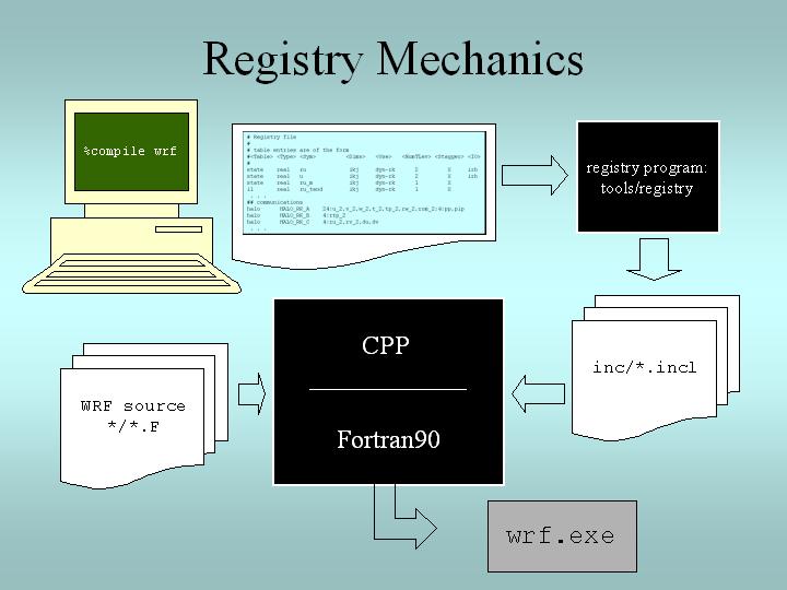
Figure 8.1. When the user compiles WRF, the Registry Program reads Registry/Registry, producing auto-generated sections of code that are stored in files in the inc directory. These are included into WRF using the CPP preprocessor and the Fortran compiler.

In addition to the WRF model itself, the Registry/Registry file is used to build the accompanying preprocessors such as real.exe (for real data) or ideal.exe (for ideal simulations), and the ndown.exe program (used for one-way, off-line nesting).

Every variable that is an input or an output field is described in the Registry. Additionally, every variable that is required for parallel communication, specifically associated with a physics package, or needs to provide a tendency to multiple physics or dynamics routines is contained in the Registry. For each of these variables, the index ordering, horizontal and vertical staggering, feedback and nesting interpolation requirements, and the associated IO are defined. For most users, to add a variable into the model requires, regardless of dimensionality, only the addition of a single line to the Registry (make sure that changes are made to the correct Registry.core file, as changes to the Registry file itself are overwritten). Since the Registry modifies code for compile-time options, any change to the Registry REQUIRES that the code be returned to the original unbuilt status with the clean –a command.

The other very typical activity for users is to define new run-time options, which are handled via a Fortran namelist file namelist.input in WRF. As with the model state arrays and variables, the entire model configuration is described in the Registry. As with the model arrays, adding a new namelist entry is as easy as adding a new line in the Registry.

While the model state and configuration are, by far, the most commonly used features in the Registry, the data dictionary has several other powerful uses. The Registry file provides input to generate all of the communications for the distributed memory processing (halo interchanges between patches, support for periodic lateral boundaries, and array transposes for FFTs to be run in the X, Y, or Z directions). The Registry associates various fields with particular physics packages so that the memory footprint reflects the actual selection of the options, not a maximal value.

Together, these capabilities allow a large portion of the WRF code to be automatically generated. Any code that is automatically generated relieves the developer of the effort of coding and debugging that portion of software. Usually, the pieces of code that are suitable candidates for automation are precisely those that are fraught with “hard to detect” errors, such as communications, indexing, and IO, which must be replicated for hundreds of variables.

Registry Syntax:

Each entry in the Registry is for a specific variable, whether it is for a new dimension in the model, a new field, a new namelist value, or even a new communication. For readability, a single entry may be spread across several lines with the traditional “\” at the end of a line to denote that the entry is continuing. When adding to the Registry, most users find that it is helpful to copy an entry that is similar to the anticipated new entry, and then modify that Registry entry. The Registry is not sensitive to spatial formatting. White space separates identifiers in each entry.

Note: Do not simply remove an identifier and leave a supposed token blank, use the appropriate default value (currently a dash character “-“).

Registry Entries:

The WRF Registry has the following types of entries (not case dependent):

Dimspec – Describes dimensions that are used to define arrays in the model

State – Describes state variables and arrays in the domain structure

I1 – Describes local variables and arrays in solve

Typedef – Describes derived types that are subtypes of the domain structure

Rconfig – Describes a configuration (e.g. namelist) variable or array

Package – Describes attributes of a package (e.g. physics)

Halo – Describes halo update interprocessor communications

Period – Describes communications for periodic boundary updates

Xpose – Describes communications for parallel matrix transposes

include – Similar to a CPP #include file

These keywords appear as the first word in a line of the file Registry to define which type of information is being provided. Following are examples of the more likely Registry types that users will need to understand.

Registry Dimspec:

The first set of entries in the Registry is the specifications of the dimensions for the fields to be defined. To keep the WRF system consistent between the dynamical cores and Chemistry, a unified registry.dimspec file is used (located in the Registry directory). This single file is included into each Registry file, with the keyword include. In the example below, three dimensions are defined: i, j, and k. If you do an “ncdump -h” on a WRF file, you will notice that the three primary dimensions are named as “west_east”, “south_north”, and “bottom_top”. That information is contained in this example (the example is broken across two lines, but interleaved).

#<Table> <Dim> <Order> <How defined>
dimspec    i      1     standard_domain
dimspec    j      3     standard_domain
dimspec    k      2     standard_domain

<Coord-axis> <Dimname in Datasets>
x          west_east
y          south_north
z          bottom_top

The WRF system has a notion of horizontal and vertical staggering, so the dimension names are extended with a “_stag” suffix for the staggered sizes. The list of names in the <Dim> column may either be a single unique character (for release 3.0.1.1 and prior), or the <Dim> column may be a string with no embedded spaces (such as my_dim). When this dimension is used later to dimension-ize a state or i1 variable, it must be surrounded by curly braces (such as {my_dim}). This <Dim> variable is not case specific, so for example “i” is the same as an entry for “I”.

Registry State and I1:

A state variable in WRF is a field that is eligible for IO and communications, and exists for the duration of the model forecast. The I1 variables (intermediate level one) are typically thought of as tendency terms, computed during a single model time-step, and then discarded prior to the next time-step. The space allocation and de-allocation for these I1 variables is automatic (on the stack for the model solver). In this example, for readability, the column titles and the entries are broken into multiple interleaved lines, with the user entries in a bold font.

Some fields have simple entries in the Registry file. The following is a state variable that is a Fortran type real. The name of the field inside the WRF model is u_gc. It is a three dimension array (igj). This particular field is only for the ARW core (dyn_em). It has a single time level, and is staggered in the X and Z directions. This field is input only to the real program (i1). On output, the netCDF name is UU, with the accompanying description and units provided.

#<Table> <Type> <Sym> <Dims>
state real u_gc igj

<Use> <NumTLev> <Stagger> <IO>
dyn_em 1 XZ i1

<DNAME> <DESCRIP> <UNITS>
"UU" "x-wind component" "m s-1"

If a variable is not staggered, a “-“ (dash) is inserted instead of leaving a blank space. The same dash character is required to fill in a location when a field has no IO specification. The variable description and units columns are used for post-processing purposes only; this information is not directly utilized by the model.

When adding new variables to the Registry file, users are warned to make sure that variable names are unique. The <Sym> refers to the variable name inside the WRF model, and it is not case sensitive. The <DNAME> is quoted, and appears exactly as typed. Do not use imbedded spaces. While it is not required that the <Sym> and <DNAME> use the same character string, it is highly recommended. The <DESCRIP> and the <UNITS> are optional, however they are a good way to supply self-documenation to the Registry. Since the <DESCRIP> value is used in the automatic code generation, restrict the variable description to 40 characters or less.

From this example, we can add new requirements for a variable. Suppose that the variable to be added is not specific to any dynamical core. We would change the <Use> column entry of dyn_em to misc (for miscellaneous). The misc entry is typical of fields used in physics packages. Only dynamics variables have more than a single time level, and this introductory material is not suitable for describing the impact of multiple time periods on the registry program. For the <Stagger> option, users may select any subset from {X, Y, Z} or {-}, where the dash character “-“ signifies “no staggering”. For example, in the ARW model, the x-direction wind component, u, is staggered in the X direction, and the y-direction wind component, v, is staggered in the Y direction.

The <IO> column handles file input and output, and it handles the nesting specification for the field. The file input and output uses three letters: i (input), r (restart), and h (history). If the field is to be in the input file to the model, the restart file from the model, and the history file from the model, the entry would be irh. To allow more flexibility, the input and history fields are associated with streams. The user may specify a digit after the i or the h token, stating that this variable is associated with a specified stream (1 through 9) instead of the default (0). A single variable may be associated with multiple streams. Once any digit is used with the i or h tokens, the default 0 stream must be explicitly stated. For example, <IO> entry i and <IO> entry i0 are the same. However, <IO> entry h1 outputs the field to the first auxiliary stream, but does not output the field to the default history stream. The <IO> entry h01 outputs the field to both the default history stream and the first auxiliary stream. For streams larger than a single digit, such as stream number thirteen, the multi-digit numerical value is enclosed inside braces: i{13}. The maximum stream is currently 24 for both input and history.

Nesting support for the model is also handled by the <IO> column. The letters that are parsed for nesting are: u (up as in feedback up), d (down, as in downscale from coarse to fine grid), f (forcing, how the lateral boundaries are processed), and s (smoothing). As with other entries, the best coarse of action is to find a field nearly identical to the one that you are inserting into the Registry file, and copy that line. The user needs to make the determination whether or not it is reasonable to smooth the field in the area of the coarse grid, where the fine-grid feeds back to the coarse grid. Variables that are defined over land and water, non-masked, are usually smoothed. The lateral boundary forcing is primarily for dynamics variables, and is ignored in this overview presentation. For non-masked fields (such as wind, temperature, & pressure), the downward interpolation (controlled by d) and the feedback (controlled by u) use default routines. Variables that are land fields (such as soil temperature TSLB) or water fields (such as sea ice XICE) have special interpolators, as shown in the examples below (again, interleaved for readability):

#<Table> <Type> <Sym> <Dims>
state real TSLB ilj
state real XICE ij

<Use> <NumTLev> <Stagger>
misc 1 Z
misc 1 -

<IO>
i02rhd=(interp_mask_land_field:lu_index)u=(copy_fcnm) i0124rhd=(interp_mask_water_field:lu_index)u=(copy_fcnm)

<DNAME> <DESCRIP>           <UNITS>
"TSLB"   "SOIL TEMPERATURE"   "K"
"SEAICE" "SEA ICE FLAG"       ""

Note that the d and u entries in the <IO> section are followed by an “=” then a parenthesis-enclosed subroutine, and a colon-separated list of additional variables to pass to the routine. It is recommended that users follow the existing pattern: du for non-masked variables, and the above syntax for the existing interpolators for masked variables.

Registry Rconfig:

The Registry file is the location where the run-time options to configure the model are defined. Every variable in the ARW namelist is described by an entry in the Registry file. The default value for each of the namelist variables is as assigned in the Registry. The standard form for the entry for two namelist variables is given (broken across lines and interleaved):

#<Table> <Type>    <Sym>
rconfig integer    run_days
rconfig integer    start_year

<How set>          <Nentries>   <Default>
namelist,time_control      1           0
namelist,time_control max_domains    1993

The keyword for this type of entry in the Registry file is rconfig (run-time configuration). As with the other model fields (such as state and i1), the <Type> column assigns the Fortran kind of the variable: integer, real, or logical. The name of the variable in ARW is given in the <Sym> column, and is part of the derived data type structure, as are the state fields. There are a number of Fortran namelist records in the file namelist.input. Each namelist variable is a member of one of the specific namelist records. The previous example shows that run_days and start_year are both members of the time_control record. The <Nentries> column refers to the dimensionality of the namelist variable (number of entries). For most variables, the <Nentries> column has two eligible values, either 1 (signifying that the scalar entry is valid for all domains) or max_domains (signifying that the variable is an array, with a value specified for each domain). Finally, a default value is given. This permits a namelist entry to be removed from the namelist.input file if the default value is acceptable.

The registry program constructs two subroutines for each namelist variable: one to retrieve the value of the namelist variable, and the other to set the value. For an integer variable named my_nml_var, the following code snippet provides an example of the easy access to the namelist variables.

INTEGER :: my_nml_var, dom_id
CALL nl_get_my_nml_var ( dom_id , my_nml_var )

The subroutine takes two arguments. The first is the input integer domain identifier (for example, 1 for the most coarse grid, 2 for the second domain), and the second argument is the returned value of the namelist variable. The associated subroutine to set the namelist variable, with the same argument list, is nl_set_my_nml_var. For namelist variables that are scalars, the grid identifier should be set to 1.

The rconfig line may also be used to define variables that are convenient to pass around in the model, usually part of a derived configuration (such as the number of microphysics species associated with a physics package). In this case, the <How set> column entry is derived. This variable does not appear in the namelist, but is accessible with the same generated nl_set and nl_get subroutines.

Registry Halo, Period, and Xpose:

The distributed memory, inter-processor communications are fully described in the Registry file. An entry in the Registry constructs a code segment which is included (with cpp) in the source code. Following is an example of a halo communication (split across two lines and interleaved for readability).

#<Table> <CommName> <Core>

halo HALO_EM_D2_3 dyn_em

<Stencil:varlist>

24:u_2,v_2,w_2,t_2,ph_2;24:moist,chem,scalar;4:mu_2,al

The keyword is halo. The communication is named in the <CommName> column, so that it can be referenced in the source code. The entry in the <CommName> column is case sensitive (the convention is to start the name with HALO_EM). The selected dynamical core is defined in the <Core> column. There is no ambiguity, as every communication in each Registry file will have the exact same <Core> column option. The last set of information is the <Stencil:varlist>. The portion in front of the “:” is the stencil size, and the comma-separated list afterwards defines the variables that are communicated with that stencil size. Different stencil sizes are available, and are “;” -separated in the same <Stencil:varlist> column. The stencil sizes 8, 24, 48 all refer to a square with an odd number of grid cells on a side, with the center grid cell removed (8 = 3x3-1, 24 = 5x5-1, 48 = 7x7-1). The special small stencil 4 is just a simple north, south, east, west communication pattern.

The convention in the WRF model is to provide a communication immediately after a variable has been updated. The communications are restricted to the mediation layer (an intermediate layer of the software that is placed between the framework level and the model level). The model level is where developers spend most of their time. The majority of users will insert communications into the dyn_em/solve_em.F subroutine. The HALO_EM_D2_3 communication, defined in the Registry file in the example above, is activated by inserting a small section of code that includes an automatically generated code segment into the solve routine, via standard cpp directives.

#ifdef DM_PARALLEL

# include "HALO_EM_D2_3.inc"

#endif

The parallel communications are only required when the ARW code is built for distributed-memory parallel processing, which accounts for the surrounding #ifdef.

The period communications are required when periodic lateral boundary conditions are selected. The Registry syntax is very similar for period and halo communications, but the stencil size refers to how many grid cells to communicate, in a direction that is normal to the periodic boundary.

#<Table> <CommName> <Core> <Stencil:varlist>

period PERIOD_EM_COUPLE_A dyn_em 2:mub,mu_1,mu_2

The xpose (a data transpose) entry is used when decomposed data is to be re-decomposed. This is required when doing FFTs in the x-direction for polar filtering, for example. No stencil size is necessary.

#<Table> <CommName> <Core> <Varlist>

xpose XPOSE_POLAR_FILTER_T dyn_em t_2,t_xxx,dum_yyy

It is anticipated that many users will add to the the parallel communications portion of the Registry file (halo and period. It is unlikely that users will add xpose fields.

Registry Package:

The package option in the Registry file associates fields with particular physics packages. Presently, it is mandatory that all 4-D arrays be assigned. Any 4-D array that is not associated with the selected physics option at run-time is neither allocated, used for IO, nor communicated. All other 2-D and 3-D arrays are eligible for use with a package assignment, but that is not required.

The purpose of the package option is to allow users to reduce the memory used by the model, since only “necessary” fields are processed. An example for a microphysics scheme is given below.

#<Table> <PackageName> <NMLAssociated> <Variables>

package kesslerscheme mp_physics==1 - moist:qv,qc,qr

The entry keyword is package, and is associated with the single physics option listed under <NMLAssociated>. The package is referenced in the code in Fortran IF and CASE statements by the name given in the <PackageName> column, instead of the more confusing and typical IF ( mp_physics == 1 ) approach. The <Variables> column must start with a dash character and then a blank “- “ (for historical reasons of backward compatibility). The syntax of the <Variables> column then is a 4-D array name, followed by a colon, and then a comma-separated list of the 3-D arrays constituting that 4-D amalgamation. In the example above, the 4-D array is moist, and the selected 3-D arrays are qv, qc, and qr. If more than one 4-D array is required, a “;” separates those sections from each other in the <Variables> column.

In addition to handling 4-D arrays and their underlying component, 3-D arrays, the package entry is able to associate generic state variables, as shown in the example following. If the namelist variable use_wps_input is set to 1, then the variables u_gc and v_gc are available to be processed.

#<Table> <PackageName> <NMLAssociated> <Variables>

package realonly use_wps_input==1 - state:u_gc,v_gc

I/O Applications Program Interface (I/O API)

The software that implements WRF I/O, like the software that implements the model in general, is organized hierarchically, as a “software stack” (http://www2.mmm.ucar.edu/wrf/WG2/Tigers/IOAPI/IOStack.html). From top (closest to the model code itself) to bottom (closest to the external package implementing the I/O), the I/O stack looks like this:

· Domain I/O (operations on an entire domain)

· Field I/O (operations on individual fields)

· Package-neutral I/O API

· Package-dependent I/O API (external package)

The lower-levels of the stack, associated with the interface between the model and the external packages, are described in the I/O and Model Coupling API specification document on http://www2.mmm.ucar.edu/wrf/WG2/Tigers/IOAPI/index.html.

Timekeeping

Starting times, stopping times, and time intervals in WRF are stored and manipulated as Earth System Modeling Framework (ESMF) time manager objects. This allows exact representation of time instants and intervals as integer numbers of years, months, hours, days, minutes, seconds, and fractions of a second (numerator and denominator are specified separately as integers). All time computations involving these objects are performed exactly by using integer arithmetic, with the result that there is no accumulated time step drift or rounding, even for fractions of a second.

The WRF implementation of the ESMF Time Manger is distributed with WRF in the external/esmf_time_f90 directory. This implementation is entirely Fortran90 (as opposed to the ESMF implementation in C++) and it is conformant to the version of the ESMF Time Manager API that was available in 2009.

WRF source modules and subroutines that use the ESMF routines do so by use-association of the top-level ESMF Time Manager module, esmf_mod:

USE esmf_mod

The code is linked to the library file libesmf_time.a in the external/esmf_time_f90 directory.

ESMF timekeeping is set up on a domain-by-domain basis in the routine setup_timekeeping (share/set_timekeeping.F). Each domain keeps track of its own clocks and alarms. Since the time arithmetic is exact there is no problem with clocks on separate domains getting out of synchronization.

Software Documentation

Detailed and comprehensive documentation aimed at WRF software is available at http://www2.mmm.ucar.edu/wrf/WG2/software_2.0.

Performance

Benchmark information is available at https://www2.mmm.ucar.edu/wrf/users/benchmark/benchdata_v422.html.