WRF Data Assimilation (WRFDA)
Data assimilation is a technique by which observations are combined with an Numerical Weather Prediciton (NWP) product (the first guess or background forecast) and their respective error statistics to provide an improved estimate (the analysis) of the atmospheric (or oceanic, Jovian, etc.) state. Variational (Var) data assimilation achieves this through iterative minimization of a prescribed cost (or penalty) function. Differences between the analysis and observations/first guess are penalized (damped) according to their perceived error. The difference between three-dimensional (3D-Var) and four-dimensional (4D-Var) data assimilation is the use of a numerical forecast model in the latter.
NSF NCAR’s Mesoscal and Microscale Meteorology (MMM) laboratory provides a unified (global/regional, multi-model, 3/4D-Var) model-space data assimilation system (WRFDA) that is freely available to the general community, along with further documentation and test results from the WRFDA Users’ site_.
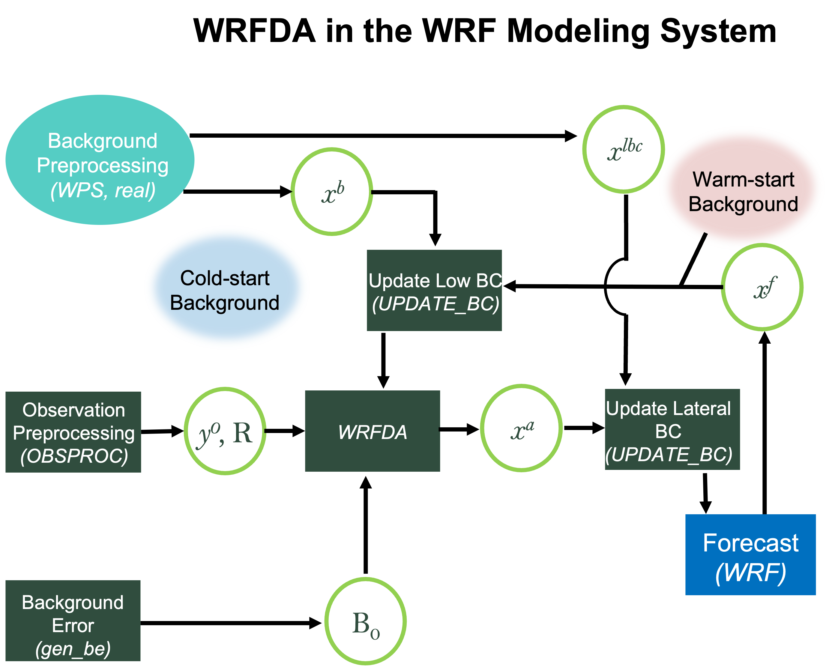
Various components of the WRFDA system are shown in the sketch below, along with their relationship with the components of the basic WRF system.
Note
- The following data are not processed by OBSPROC:
Radar precipitation data in ASCII format (requires separate pre-processing)
Conventional observations in PREPBUFR format
Radiance GPSRO in BUFR format
x b
first guess, either from a previous WRF forecast or from WPS or real.exe output
x lbc
lateral boundary from WPS or real.exe output
x a
analysis from the WRFDA data assimilation system
x f
WRF forecast output
y o
observations processed by OBSPROC; note: PREPBUFR input, radar, radiance, and rainfall data do not go through OBSPROC
B 0
background error statistics from generic BE data (CV3) or gen_be
R
observational and representative error statistics
This chapter provides instructions for installing and running the various components of the WRFDA system. For training purposes, a test case is proviced that includes the following input data:
observation files
a netCDF background file (WPS or real.exe output, the first guess of the analysis)
- background error statistics (estimate of errors in the background file)
Download this tutorial data set, which is described later in more detail. Outside of the tutorial, these files must be created by the user. See Running Observation Preprocessor (OBSPROC) for creating observation files. See Background Error (BE) and Running GEN_BE for generating a background error statistics file, if using cv_options=5, 6, or 7.
Before trying a case with user-created data, it is suggested to first run the WRFDA-related programs using the supplied test case. This provides the opportunity to learn how to run the programs with pre-tested data, and to establish whether the computing environment is capable of running the entire data assimilation system.
Note
WARNING: It is impossible to test every permutation of computer, compiler, number of processors, case, namelist option, etc. for every WRFDA release. Supported namelist (default) options are indicated in WRFDA/var/README.namelist.
As a professional courtesy, the following references should be included in any publication that uses any component of the community WRFDA system
Barker, D.M., W. Huang, Y.R. Guo, and Q.N. Xiao., 2004: A Three-Dimensional (3DVAR) Data Assimilation System For Use With MM5: Implementation and Initial Results. Mon. Wea. Rev., 132, 897-914.
A Fortran 90 compiler is required to run WRFDA, and WRFDA can be compiled on the following platforms. Note that it is not recommended to make modifications to the configure file used to compile WRFDA.
Linux (ifort, gfortran, pgf90)
Macintosh (gfortran, ifort)
IBM (xlf)
SGI Altix (ifort)
Installing WRFDA
The following instructions describe how to obtain all source code, including that for 3dvar, 4dvar, and WRFPLUS.
Obtaining WRFDA Source Code
Start by Downloading the WRF source code, which includes the WRFDA and WRFPLUS systems.
Note
Although WRF and WRFDA source code are packaged together, they can not be built together. They must be built in a separate directory.
Click on “New User” and become a registered user. After confirming the email address, log in to access the code, which is available on GitHub. The WRF code can either be obtained with a
git clone...command, or by downloading a zipped file.
After the code is cloned from GitHub, or downloaded and unpacked (e.g.,
unzip WRFVX.X.zip), a new directory, WRF, should exist that contains the WRFDA source, the WRFPLUS source (now fully integrated into WRF and TLM/ADJ code, located under the wrftladj directory), external libraries, and fixed files. The following is a list of the system components and content for each subdirectory:
Directory Name |
Content |
|---|---|
var/da |
WRFDA source code |
var/run |
Fixed input files required by WRFDA, such as background error covariance |
radiance-related files |
CRTM coefficients and VARBC.in |
var/external |
Libraries needed by WRFDA, includes CRTM, BUFR, LAPACK, BLAS |
var/obsproc |
OBSPROC source code, namelist, and observation error files |
var/gen_be |
Source code of gen_be, the utility to create background error statistics files |
var/build |
Builds all .exe files |
Build WRFDA Libraries
Some external libraries (e.g., LAPACK, BLAS, and NCEP BUFR) are included with WRF source code. To compile WRFDA, the only mandatory library is netCDF.
Note
Make sure all required libraries were compiled using the same compiler that will be used to build WRFDA, since the libraries produced by one compiler may not be compatible with code compiled with another.
The environment variable NETCDF must be set, pointing to the directory where the netCDF library is installed.
> setenv NETCDF path-to-netcdf-library/netcdfThe source code for BUFRLIB 10.2.3 (with minor modifications) is included with the WRF source code, and is compiled automatically. This library is used for assimilating files in PREPBUFR and NCEP BUFR format.
AMSR2 data can be assimilated in HDF5 format, and requires that HDF5 libraries are installed (download them from the HDF Group). To use HDF5 in WRFDA, the environment variable HDF5 must point to the path to the HDF5 build. For e.g.,
> setenv HDF5 hdf5_pathThe HDF5 path should contain the directories include and lib. Some platforms may require an additional environment variable setting for LD_LIBRARY_PATH, that points to the HDF5 lib directory. For e.g.,
> setenv LD_LIBRARY_PATH ${LD_LIBRARY_PATH}:hdf5_path/libIf satellite radiance data are to be used, a Radiative Transfer Model (RTM) is required. The RTM versions that WRFDA supports are CRTM V2.3.0 and RTTOV V12.1.
CRTM V2.3.0 source code is included with the WRF source code, and is compiled automatically. CRTM Coefficients can be downloaded from the WRFDA CRTM Coefficients page.
To use RTTOV, download and install the RTTOV v12 library before compiling WRFDA. The RTTOV libraries must be compiled with the ‘emis_atlas’ option in order to work with WRFDA; see the RTTOV “readme.txt” for instructions. After compiling RTTOV (see the RTTOV documentation for detailed instructions), set the RTTOV environment variable to the path where the lib directory resides. For example, if the library files can be found in /usr/local/rttov11/gfortran/lib/librttov11..a*,
> setenv RTTOV /usr/local/rttov11/gfortran
Compile WRFDA for 3D-Var and 4D-Var
Assuming all required libraries are installed correctly, WRFDA can be built for a 3D-var simulation, a 4D-var simulation, or for both.
For organization and consistency, rename the WRF directory.
> mv WRF WRFDANote
If both 3DVAR and 4DVAR are going to be run, it is not necessary to compile the code twice. The da_wrfvar.exe executable compiled for 4DVAR can be used for both 3DVAR and 4DVAR assimilation.
If planning to run a 4D-var simulation, WRFPLUS must be built prior to building WRFDA. If WRFDA 4D-var will not be used, skip ahead to Configure WRFDA.
WRFPLUS Install
To run WRFDA 4DVAR, WRFPLUS must first be installed. WRFPLUS contains the adjoint and tangent linear models, based on a simplified WRF model, which includes a few simplified physics packages, such as surface drag, large scale condensation and precipitation, and cumulus parameterization.
WRFPLUS code is fully integrated into WRF and TLM/ADJ code, and is located in the wrftladj directory. Obtain the WRF source code by cloning it from GitHub, or by downloading the packaged file.
Once the code has been obtained (and unpacked, if downloading), rename the new ‘WRF’ directory appropriately to WRFPLUS, and then run the configure script.
> mv WRF WRFPLUS
> cd WRFPLUS
> ./configure wrfplus
As with 3D-Var, serial means single-processor, and dmpar means Distributed Memory Parallel (MPI). Choose the same option for WRFPLUS that will be used for WRFDA.
Compile WRFPLUS
> ./compile wrfplus >& compile.out
> ls -ls main/*.exe
If compilation was successful, there should now be a WRFPLUS executable (wrfplus.exe).
53292 -rwxr-xr-x 1 user man 54513254 Apr 6 22:43 main/wrfplus.exeFinally, set the environment variable WRFPLUS_DIR to the appropriate directory:
>setenv WRFPLUS_DIR ${source_code_directory}/WRFPLUS
Configure WRFDA
Configuring the code differs depending on whether the install will be for 3dvar or 4dvar simulating. If planning to use both, then use the configure steps for 4dvar, as the 4dvar build allows simulating with 3dvar.
Enter the WRFDA directory and run the configure script.
3d-Var Configuration
> cd WRFDA
> ./configure wrfda
4d-Var Configuation
To use RTTOV to assimilate radiance data, the appropriate environment variable must be set prior to compiling. See the previous Installing WRFDA section for instructions.> cd WRFDA > ./configure 4dvar
A list of configuration options should appear. Each option combines an operating system, a compiler type, and a parallelism option. Since the configuration script does not check which compilers are actually installed on the system, be sure to select an option that is available. The available parallelism options are single-processor (serial), shared-memory parallel (smpar), distributed-memory parallel (dmpar), and distributed-memory with shared-memory parallel (sm+dm). However, beginning with WRFDA Version 4.1, shared-memory (smpar and sm+dm) options are no longer recommended. The above command will produce something similar to the following.
checking for perl5... no
checking for perl... found /usr/bin/perl (perl)
Will use NETCDF in dir: /glade/apps/opt/netcdf/4.3.0/gnu/4.8.2/
Will use HDF5 in dir: /glade/u/apps/opt/hdf5/1.8.12/gnu/4.8.2/
PHDF5 not set in environment. Will configure WRF for use without.
Will use 'time' to report timing information
$JASPERLIB or $JASPERINC not found in environment, configuring to build without grib2 I/O...
------------------------------------------------------------------------
Please select from among the following Linux x86_64 options:

  1. (serial)   2. (smpar)   3. (dmpar)   4. (dm+sm)   PGI (pgf90/gcc)
  5. (serial)   6. (smpar)   7. (dmpar)   8. (dm+sm)   PGI (pgf90/pgcc): SGI MPT
  9. (serial)  10. (smpar)  11. (dmpar)  12. (dm+sm)   PGI (pgf90/gcc): PGI accelerator
 13. (serial)  14. (smpar)  15. (dmpar)  16. (dm+sm)   INTEL (ifort/icc)
             17. (dm+sm)   INTEL (ifort/icc): Xeon Phi (MIC architecture)
 18. (serial)  19. (smpar)  20. (dmpar)  21. (dm+sm)   INTEL (ifort/icc): Xeon (SNB with AVX mods)
 22. (serial)  23. (smpar)  24. (dmpar)  25. (dm+sm)   INTEL (ifort/icc): SGI MPT
 26. (serial)  27. (smpar)  28. (dmpar)  29. (dm+sm)   INTEL (ifort/icc): IBM POE
 30. (serial)               31. (dmpar)                PATHSCALE (pathf90/pathcc)
 32. (serial)  33. (smpar)  34. (dmpar)  35. (dm+sm)   GNU (gfortran/gcc)
 36. (serial)  37. (smpar)  38. (dmpar)  39. (dm+sm)   IBM (xlf90_r/cc_r)
 40. (serial)  41. (smpar)  42. (dmpar)  43. (dm+sm)   PGI (ftn/gcc): Cray XC CLE
 44. (serial)  45. (smpar)  46. (dmpar)  47. (dm+sm)   CRAY CCE (ftn/cc): Cray XE and XC
 48. (serial)  49. (smpar)  50. (dmpar)  51. (dm+sm)   INTEL (ftn/icc): Cray XC
 52. (serial)  53. (smpar)  54. (dmpar)  55. (dm+sm)   PGI (pgf90/pgcc)
 56. (serial)  57. (smpar)  58. (dmpar)  59. (dm+sm)   PGI (pgf90/gcc): -f90=pgf90
 60. (serial)  61. (smpar)  62. (dmpar)  63. (dm+sm)   PGI (pgf90/pgcc): -f90=pgf90
 64. (serial)  65. (smpar)  66. (dmpar)  67. (dm+sm)   INTEL (ifort/icc): HSW/BDW
 68. (serial)  69. (smpar)  70. (dmpar)  71. (dm+sm)   INTEL (ifort/icc): KNL MIC

Enter selection [1-71] : 34
------------------------------------------------------------------------

Configuration successful!
------------------------------------------------------------------------
... ...
After entering an appropriate option, the configure script should print the message Configuration successful! followed by some detailed configuration information.
Note
Depending on the system, a warning message may appear stating that some Fortran 2003 features have been removed - this message is normal and can be ignored. However, if the message “One of compilers testing failed! Please check your compiler,” appears, configuration has probably failed, likely due to an incompatible option being chosen.
After running the configuration script and choosing a compilation option, a configure.wrf file is created. Because of the variety of ways that a computer can be configured, if the WRFDA build ultimately fails, there is a chance that minor modifications to the configure.wrf file may be necessary.
Compile WRFDA
Regardless of whether compiling WRFDA for a 3dvar or 4dvar simulation, the command will be the same.
> ./compile all_wrfvar >& compile.out
A successful compile produces 44 executables - 43 of which are in the var/build directory and linked to the var/da directory, with the 44th, obsproc.exe, found in the var/obsproc/src directory. The executables can be listed with the following command:
>ls -l var/build/*exe var/obsproc/src/obsproc.exe

-rwxr-xr-x 1 user   885143 Apr  4 17:22 var/build/da_advance_time.exe
-rwxr-xr-x 1 user  1162003 Apr  4 17:24 var/build/da_bias_airmass.exe
-rwxr-xr-x 1 user  1143027 Apr  4 17:23 var/build/da_bias_scan.exe
-rwxr-xr-x 1 user  1116933 Apr  4 17:23 var/build/da_bias_sele.exe
-rwxr-xr-x 1 user  1126173 Apr  4 17:23 var/build/da_bias_verif.exe
-rwxr-xr-x 1 user  1407973 Apr  4 17:23 var/build/da_rad_diags.exe
-rwxr-xr-x 1 user  1249431 Apr  4 17:22 var/build/da_tune_obs_desroziers.exe
-rwxr-xr-x 1 user  1186368 Apr  4 17:24 var/build/da_tune_obs_hollingsworth1.exe
-rwxr-xr-x 1 user  1083862 Apr  4 17:24 var/build/da_tune_obs_hollingsworth2.exe
-rwxr-xr-x 1 user  1193390 Apr  4 17:24 var/build/da_update_bc_ad.exe
-rwxr-xr-x 1 user  1245842 Apr  4 17:23 var/build/da_update_bc.exe
-rwxr-xr-x 1 user  1492394 Apr  4 17:24 var/build/da_verif_grid.exe
-rwxr-xr-x 1 user  1327002 Apr  4 17:24 var/build/da_verif_obs.exe
-rwxr-xr-x 1 user 26031927 Apr  4 17:31 var/build/da_wrfvar.exe
-rwxr-xr-x 1 user  1933571 Apr  4 17:23 var/build/gen_be_addmean.exe
-rwxr-xr-x 1 user  1944047 Apr  4 17:24 var/build/gen_be_cov2d3d_contrib.exe
-rwxr-xr-x 1 user  1927988 Apr  4 17:24 var/build/gen_be_cov2d.exe
-rwxr-xr-x 1 user  1945213 Apr  4 17:24 var/build/gen_be_cov3d2d_contrib.exe
-rwxr-xr-x 1 user  1941439 Apr  4 17:24 var/build/gen_be_cov3d3d_bin3d_contrib.exe
-rwxr-xr-x 1 user  1947331 Apr  4 17:24 var/build/gen_be_cov3d3d_contrib.exe
-rwxr-xr-x 1 user  1931820 Apr  4 17:24 var/build/gen_be_cov3d.exe
-rwxr-xr-x 1 user  1915177 Apr  4 17:24 var/build/gen_be_diags.exe
-rwxr-xr-x 1 user  1947942 Apr  4 17:24 var/build/gen_be_diags_read.exe
-rwxr-xr-x 1 user  1930465 Apr  4 17:24 var/build/gen_be_ensmean.exe
-rwxr-xr-x 1 user  1951511 Apr  4 17:24 var/build/gen_be_ensrf.exe
-rwxr-xr-x 1 user  1994167 Apr  4 17:24 var/build/gen_be_ep1.exe
-rwxr-xr-x 1 user  1996438 Apr  4 17:24 var/build/gen_be_ep2.exe
-rwxr-xr-x 1 user  2001400 Apr  4 17:24 var/build/gen_be_etkf.exe
-rwxr-xr-x 1 user  1942988 Apr  4 17:24 var/build/gen_be_hist.exe
-rwxr-xr-x 1 user  2021659 Apr  4 17:24 var/build/gen_be_stage0_gsi.exe
-rwxr-xr-x 1 user  2012035 Apr  4 17:24 var/build/gen_be_stage0_wrf.exe
-rwxr-xr-x 1 user  1973193 Apr  4 17:24 var/build/gen_be_stage1_1dvar.exe
-rwxr-xr-x 1 user  1956835 Apr  4 17:24 var/build/gen_be_stage1.exe
-rwxr-xr-x 1 user  1963314 Apr  4 17:24 var/build/gen_be_stage1_gsi.exe
-rwxr-xr-x 1 user  1975042 Apr  4 17:24 var/build/gen_be_stage2_1dvar.exe
-rwxr-xr-x 1 user  1938468 Apr  4 17:24 var/build/gen_be_stage2a.exe
-rwxr-xr-x 1 user  1952538 Apr  4 17:24 var/build/gen_be_stage2.exe
-rwxr-xr-x 1 user  1202392 Apr  4 17:22 var/build/gen_be_stage2_gsi.exe
-rwxr-xr-x 1 user  1947836 Apr  4 17:24 var/build/gen_be_stage3.exe
-rwxr-xr-x 1 user  1928353 Apr  4 17:24 var/build/gen_be_stage4_global.exe
-rwxr-xr-x 1 user  1955622 Apr  4 17:24 var/build/gen_be_stage4_regional.exe
-rwxr-xr-x 1 user  1924416 Apr  4 17:24 var/build/gen_be_vertloc.exe
-rwxr-xr-x 1 user  2057673 Apr  4 17:24 var/build/gen_mbe_stage2.exe
-rwxr-xr-x 1 user  2110993 Apr  4 17:32 var/obsproc/src/obsproc.exe
The primary executable for running WRFDA is da_wrfvar.exe. Make sure it has been created after the compilation: it is not uncommon for all executables, except for this one, to be successfully compiled. If this occurs, check the compilation log file for errors.
The basic gen_be utility for the regional model consists of gen_be_stage0_wrf.exe, gen_be_stage1.exe, gen_be_stage2.exe, gen_be_stage2a.exe, gen_be_stage3.exe, gen_be_stage4_regional.exe, and gen_be_diags.exe.
da_update_bc.exe is used to update update the WRF lower and lateral boundary conditions before and after a new WRFDA analysis is generated. This is detailed in Updating WRF Boundary Conditions.
da_advance_time.exe is a useful tool for date/time manipulation. Issue
$WRFDA_DIR/var/build/da_advance_time.exeto see its usage instructions.obsproc.exe prepares conventional observations for WRFDA assimilation. Its use is detailed in Running Observation Preprocessor (OBSPROC).
If CRTM will be used for radiance assimilation, check $WRFDA_DIR/var/external/crtm_2.3.0/libsrc to ensure that libCRTM.a was generated.
Clean Old Compilation
To remove all object files and executables, issue the command:
> ./clean
To remove all build files, including configure.wrf, issue the command:
> ./clean -a
The clean -a command is recommended if the compilation fails, or if the configuration file has been modified and the default settings need to be restored.
Running Observation Preprocessor (OBSPROC)
The OBSPROC program reads observations in LITTLE_R text-based format. Observations are provided for the tutorial case, but otherwise it is the user’s responsiblity to prepare the observation files. Sources of freely-available observations are available from the WRFDA Free Data page, which also includes instructions for converting observations to LITTLE_R format, since raw observation files are available in a multitude of formats, such as ASCII, BUFR, PREPBUFR, MADIS (see Converter for MADIS to LITTLE_R), and HDF. A more complete description of the LITTLE_R format, as well as conventional observation data sources for WRFDA, are available from the LITTLE_R Help page, the Observation Pre-processing for WRFDA presentation, or by referencing the OBSGRID section of the WRF Utilities and Tools chapter of this Users’ Guide.
The purpose of OBSPROC is to:
Remove observations outside the specified temporal and spatial domains
Re-order and merge duplicate (in time and location) data reports
Retrieve pressure or height, based on observed information using the hydrostatic assumption
Check multi-level observations for vertical consistency and superadiabatic conditions
Assign observation errors based on a pre-specified error file
Write out the observation file to be used by WRFDA in ASCII or BUFR format
The OBSPROC program (obsproc.exe) should be in the directory $WRFDA_DIR/var/obsproc/src if compile all_wrfvar completed successfully.
Download the tutorial case, which contains example files for all the exercises in this guide.
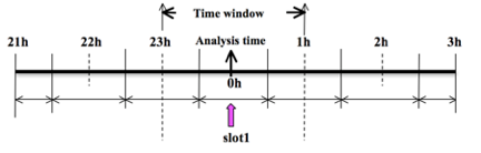
OBSPROC for 3DVAR
As an example, to prepare the observation file at the analysis time, all observations in the range +/- 1h are processed, meaning, for this example, observations between 23h and 1h are treated as the observations at 0h. This is illustrated in the following figure.
OBSPROC requires at least 3 files to run successfully:
A namelist file (namelist.obsproc)
An observation error file (obserr.txt)
One or more observation files
Optionally, a table for specifying the elevation information for marine observations over the US Great Lakes (msfc.tbl)
The files obserr.txt and msfc.tbl are included in the source code under var/obsproc. An example namelist file (namelist_obsproc.3dvar.wrfvar-tut) can be found in the var/obsproc directory. Thus, proceed as follows.
> cd $WRFDA_DIR/var/obsproc
> cp namelist.obsproc.3dvar.wrfvar-tut namelist.obsproc
Next, edit namelist.obsproc. It is likely that only variables listed under records 1, 2, 6, 7, and 8 will need modification. See $WRFDA_DIR/var/obsproc/README.namelist, or OBSPROC Namelist Variables for details. Pay attention to the record 7 and 8 variables - these determine the domain for which observations are written to the output observation file. Alternative to filtering the observations spatially, set domain_check_h=.false. under &record4.
If running the tutorial case, copy or link the sample observation file (ob/2008020512/obs.2008020512) to the obsproc directory. Alternatively, edit the namelist variable obs_gts_filename to point to the observation file’s full path.
Issue the following to run OBSPROC.
> ./obsproc.exe >& obsproc.out
Once obsproc.exe has completed successfully, an observation file with the naming convention obs_gts_YYYY-MM-DD_HH:NN:SS.3DVAR will be available in the obsproc directory. For the tutorial case, this will be obs_gts_2008-02-05_12:00:00.3DVAR. This is the observation file that will be input to WRFDA. It is an ASCII file that contains a header section (example shown below) followed by observations. Observation description and format are described in the last six lines of the header section.
TOTAL =   9066, MISS. =-888888.,
SYNOP =    757, METAR =   2416, SHIP  =    145, BUOY  =    250, BOGUS =      0,
TEMP  =     86, AMDAR =     19, AIREP =    205, TAMDAR=      0, PILOT =     85,
SATEM =    106, SATOB =   2556, GPSPW =    187, GPSZD =      0, GPSRF =      3,
GPSEP =      0, SSMT1 =      0, SSMT2 =      0, TOVS  =      0, QSCAT =   2190,
PROFL =     61, AIRSR =      0, OTHER =      0, PHIC  =  40.00, XLONC = -95.00,
TRUE1 =  30.00, TRUE2 =  60.00, XIM11 =   1.00, XJM11 =   1.00,
base_temp= 290.00, base_lapse=  50.00, PTOP  =  1000., base_pres=100000.,
base_tropo_pres= 20000., base_strat_temp=   215.,
IXC   =     60, JXC   =     90, IPROJ =      1, IDD   =      1, MAXNES=      1,
NESTIX=     60,
NESTJX=     90,
NUMC  =      1,
DIS   =  60.00,
NESTI =      1,
NESTJ =      1,
INFO  = PLATFORM, DATE, NAME, LEVELS, LATITUDE, LONGITUDE, ELEVATION, ID.
SRFC  = SLP, PW (DATA,QC,ERROR).
EACH  = PRES, SPEED, DIR, HEIGHT, TEMP, DEW PT, HUMID (DATA,QC,ERROR)*LEVELS.
INFO_FMT = (A12,1X,A19,1X,A40,1X,I6,3(F12.3,11X),6X,A40)
SRFC_FMT = (F12.3,I4,F7.2,F12.3,I4,F7.3)
EACH_FMT = (3(F12.3,I4,F7.2),11X,3(F12.3,I4,F7.2),11X,3(F12.3,I4,F7.2))
#------------------------------------------------------------------------------#
........... observations ...........
To visualize the ASCII file’s content, NCL (NCAR Command Language) scripts that display the distribution and type of observations are available. Download the WRFDA Tools Package, and then find the relevant script (plot_ob_ascii_loc.ncl) in $TOOLS_DIR/var/graphics/ncl. NCL must be installed to use this script; see the NCL site for more information about this post-processing tool.
OBSPROC for 4DVAR
To prepare the observation file, for example, at the analysis time 0h for 4D-Var, all observations from 0h to 6h will be processed and grouped in 7 sub-windows (slot1 through slot7) as illustrated in the following figure.
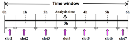
Note
‘Analysis time’ in the above figure is not the actual analysis time (0h). It indicates the time_analysis setting in the namelist, which in this example is three hours later than the actual analysis time. The actual analysis time is still 0h.
An example namelist (namelist_obsproc.4dvar.wrfvar-tut) has already been provided in the var/obsproc directory. Thus, proceed as follows:
> cd $WRFDA_DIR/var/obsproc
> cp namelist.obsproc.4dvar.wrfvar-tut namelist.obsproc
- Modify the namelist settings for the following.
time_analysis
num_slows_past
time_slots_ahead
For this tutorial case, the actual analysis time is 2008-02-05_12:00:00, but time_analysis should be set to 3 hours later. The different values of time_analysis, num_slots_past, and time_slots_ahead contribute to the actual times analyzed. For example, if time_analysis = 2008-02-05_16:00:00, num_slots_past=4, and time_slots_ahead=2, the final results will be the same as before.
Edit the domain settings to correspond with the experiment. An inclusive list of namelist options and descriptions is available in WRFDA Description of Namelist Variables. Pay attention to the record 7 and 8 variables, which determine the domain for which observations will be written to the output observation file. Alternatively, instead of filtering the observations spatially, domain_check_h=.false. can be set under &record4.
If running the tutorial case, copy or link the sample observation file (ob/2008020512/obs.2008020512) to the obsproc directory. Alternatively, edit the namelist variable obs_gts_filename to point to the observation file’s full path.
Issue the following to run OBSPROC.
> obsproc.exe >& obsproc.out
Once obsproc.exe has completed successfully, the observation data files will be available (e.g., for the tutorial case):
obs_gts_2008-02-05_12:00:00.4DVAR
obs_gts_2008-02-05_13:00:00.4DVAR
obs_gts_2008-02-05_14:00:00.4DVAR
obs_gts_2008-02-05_15:00:00.4DVAR
obs_gts_2008-02-05_16:00:00.4DVAR
obs_gts_2008-02-05_17:00:00.4DVAR
obs_gts_2008-02-05_18:00:00.4DVAR
These files are the input observations to WRF 4D-Var.
Running WRFDA
Download Test Data
The WRFDA system requires three input data files to run:
Input Data |
Format |
Created By |
|---|---|---|
First Guess |
netCDF |
WRF Preprocessing System (WPS) and real.exe (wrfinput) or WRF (wrfout) |
Observations |
ASCII (PREPBUFR or BUFR for radiance also possible) |
OBSPROC |
Background Error Statistics |
Binary |
WRFDA gen_be utility |
For the test case, store data in a directory defined by the environment variable $DAT_DIR. This directory can be in any location, and it should have read access. Issue the following.
> setenv DAT_DIR data_directoryWhere, data_directory is an example name, and is where WRFDA input data is stored.
If it does not already exist, download the sample data for the tutorial case, place it in the $*$DAT_DIR*, and extract it.
> gunzip WRFDAV4.0-testdata.tar.gz
> tar -xvf WRFDAV4.0-testdata.tar
The following files should now exist in $DAT_DIR
ob/2008020512/ob.2008020512      #  Observation data in little_r format
rc/2008020512/wrfinput_d01       #  First guess file
rc/2008020512/wrfbdy_d01         #  lateral boundary file
be/be.dat                        #  Background error file
......
Three input files (first guess, observations from OBSPROC, and background error statistics) should now exist in $DAT_DIR.
Run a 3DVAR Test Case
The data for the tutorial case is valid at 12 UTC 5 February 2008. The first guess comes from the NCEP FNL (Final) Operational Global Analysis data, and has been passed through the WPS and real.exe programs.
Create a new working directory; for e.g.,
mkdir $WRFDA_DIR/workdir
Set the environment variable WORK_DIR to this directory; for e.g.,
setenv WORK_DIR $WRFDA_DIR/workdir
Issue the following commands.
> cd $WORK_DIR
> cp $DAT_DIR/namelist.input.3dvar namelist.input
> ln -sf $WRFDA_DIR/run/LANDUSE.TBL .
> ln -sf $DAT_DIR/rc/2008020512/wrfinput_d01 ./fg
> ln -sf $DAT_DIR/ob/2008020512/obs_gts_2008-02-05_12:00:00.3DVAR ./ob.ascii
        (note the different name!)
> ln -sf $DAT_DIR/be/be.dat .
> ln -sf $WRFDA_DIR/var/da/da_wrfvar.exe .
Edit namelist.input, which is a basic namelist for the tutorial test case, as shown below.
&wrfvar1
var4d=false,
print_detail_grad=false,
/

&wrfvar2
/

&wrfvar3
ob_format=2,
/

&wrfvar4
/

&wrfvar5
/

&wrfvar6
max_ext_its=1,
ntmax=50,
orthonorm_gradient=true,
/

&wrfvar7
cv_options=5,
/

&wrfvar8
/

&wrfvar9
/

&wrfvar10
test_transforms=false,
test_gradient=false,
/

&wrfvar11
/

&wrfvar12
/

&wrfvar13
/

&wrfvar14
/

&wrfvar15
/

&wrfvar16
/

&wrfvar17
/

&wrfvar18
analysis_date="2008-02-05_12:00:00.0000",
/

&wrfvar19
/

&wrfvar20
/

&wrfvar21
time_window_min="2008-02-05_11:00:00.0000",
/

&wrfvar22
time_window_max="2008-02-05_13:00:00.0000",
/

&time_control
start_year=2008,
start_month=02,
start_day=05,
start_hour=12,
end_year=2008,
end_month=02,
end_day=05,
end_hour=12,
/

&fdda
/

&domains
e_we=90,
e_sn=60,
e_vert=41,
dx=60000,
dy=60000,
/

&dfi_control
/

&tc
/

&physics
mp_physics=3,
ra_lw_physics=1,
ra_sw_physics=1,
radt=60,
sf_sfclay_physics=1,
sf_surface_physics=1,
bl_pbl_physics=1,
cu_physics=1,
cudt=5,
num_soil_layers=5,
mp_zero_out=2,
co2tf=0,
/

&scm
/

&dynamics
/

&bdy_control
/

&grib2
/

&fire
/

&namelist_quilt
/

&perturbation
/
No edits are necessary for running the tutorial case without radiance data. If planning to use PREPBUFR-format data, change ob_format=1 in &wrfvar3 in namelist.input and link the data as ob.bufr,
> ln -fs $DAT_DIR/ob/2008020512/gdas1.t12z.prepbufr.nr ob.bufr
Issue the following to run WRFDA 3D-Var.
da_wrfvar.exe >& wrfda.log
Check wrfda.log (or rsl.out.0000, if run with distributed-memory), which contains WRFDA runtime information. Make sure the following message appears at the end.
*** WRF-Var completed successfully ***
If WRFDA was successful, the following new files are available.
namelist.output.da : contains the complete namelist settings; note that settings appearing in namelist.output.da, but not specified in namelist.input, are the default values from $WRFDA_DIR/Registry/registry.var.
wrfvar_output : the WRFDA analysis file, i.e. the new initial condition for WRF
A number of diagnostic files; text files containing various diagnostics are explained in WRFDA Diagnostics
To understand the role of various WRFDA options, re-run WRFDA after changing different namelist options, and then compare various diagnostics with an earlier run. Some examples are listed below.
Response of Convergence Criteria
&wrfvar6
eps = 0.0001,
/
Response of outer loop on minimization
&wrfvar6
max_ext_its = 2,
/
Response of outer loop on minimization
&wrfvar6
max_ext_its = 2,
/
This activates the outer loop for the minimization procedure. Note that when running multiple outer loops with the CV3 background error option, the scaling factors (as1, as2, as3, as4, as5) must be specified. More details can be found in the Modifying CV3 Length Scales and Variance section in Generic BE Option: CV3.
Response of suppressing particular types of data in WRFDA
The content included in the observation file, and in the WRFDA namelist.input settings determines the types of observations WRFDA uses. For example, if the observation file contains SYNOP data, its usage can be suppressed by setting use_synopobs=false in record &wrfvar4.
Note
It is not an problem if no SYNOP data are in the observation file, while use_synopobs=true.
Turning on and off certain types of observations is widely used for assessing the impact of observations for data assimilation. For example, make the WRFDA convergence criterion more stringent by reducing the value of EPS to e.g. 0.0001, by adding EPS=0.0001 in the namelist.input record &wrfvar6. See Additional Background Error Options for more namelist options.
Run a 4DVAR Test Case
Create a new working directory; for e.g.,
> mkdir $WRFDA_DIR/workdir
Set the WORK_DIR environment variable.
> setenv WORK_DIR $WRFDA_DIR/workdirThe tutorial case analysis date is 2008020512 and the test data directories are:
> ls -lr $DAT_DIR
ob/2008020512
ob/2008020513
ob/2008020514
ob/2008020515
ob/2008020516
ob/2008020517
ob/2008020518
rc/2008020512
be
Note
WRFDA 4D-Var is able to assimilate conventional observational, satellite radiance BUFR, and precipitation data. Input data format can be PREPBUFR or ASCII observations, processed by OBSPROC.
Link the executable file.
> cd $WORK_DIR
> ln -fs $WRFDA_DIR/var/da/da_wrfvar.exe .
Link the observational data, first guess, BE and LANDUSE.TBL, etc.
> ln -fs $DAT_DIR/ob/2008020512/ob01.ascii ob01.ascii
> ln -fs $DAT_DIR/ob/2008020513/ob02.ascii ob02.ascii
> ln -fs $DAT_DIR/ob/2008020514/ob03.ascii ob03.ascii
> ln -fs $DAT_DIR/ob/2008020515/ob04.ascii ob04.ascii
> ln -fs $DAT_DIR/ob/2008020516/ob05.ascii ob05.ascii
> ln -fs $DAT_DIR/ob/2008020517/ob06.ascii ob06.ascii
> ln -fs $DAT_DIR/ob/2008020518/ob07.ascii ob07.ascii

> ln -fs $DAT_DIR/rc/2008020512/wrfinput_d01 .
> ln -fs $DAT_DIR/rc/2008020512/wrfbdy_d01 .
> ln -fs wrfinput_d01 fg

> ln -fs $DAT_DIR/be/be.dat .
> ln -fs $WRFDA_DIR/run/LANDUSE.TBL .
> ln -fs $WRFDA_DIR/run/GENPARM.TBL .
> ln -fs $WRFDA_DIR/run/SOILPARM.TBL .
> ln -fs $WRFDA_DIR/run/VEGPARM.TBL .
> ln -fs $WRFDA_DIR/run/RRTM_DATA_DBL RRTM_DATA
> ln -fs $WRFDA_DIR/run/CAMtr_volume_mixing_ratio .
Note
CAMtr_volume_mixing_ratio is needed to run 4D-Var version 4.4+.
Copy the sample namelist.
> cp $DAT_DIR/namelist.input.4dvar namelist.input
Edit necessary namelist variables.
The most important 4D-Var namelist variables are listed below. Refer to the README.namelist file in the WRF source code, under the $WRFDA_DIR/var directory for additional information.
Note
analysis_date, time_window_min, and start_xxx in &time_control should always be equal to each other
time_window_max and end_xxx should always be equal to each other;
run_hours is the difference between start_xxx and end_xxx, which is the length of the 4D-Var time window
&wrfvar1

var4d=true,
var4d_lbc=false,
var4d_bin=3600,
/

&wrfvar18
analysis_date="2008-02-05_12:00:00.0000",
/

&wrfvar21
time_window_min="2008-02-05_12:00:00.0000",
/

&wrfvar22
time_window_max="2008-02-05_18:00:00.0000",
/

&time_control
run_hours=6,
start_year=2008,
start_month=02,
start_day=05,
start_hour=12,
end_year=2008,
end_month=02,
end_day=05,
end_hour=18,
interval_seconds=21600,
debug_level=0,
/
WRFDA 4D-Var is capable of considering lateral boundary conditions as control variables during minimization, by setting var4d_lbc=true in the namelist. To enable this option, the first guess at the beginning and end of the time window must be available.
> ln -fs $DAT_DIR/rc/2008020518/wrfinput_d01 fg02Note
This option is not recommended for WRFDA beginners, or until a good understanding of the 4D-Var lateral boundary conditions control is established. To disable this feature, make sure var4d_lbc=.false.
If PREPBUFR formatted data is being used, set ob_format=1 in the namelist.input record &wrfvar3. Because 12UTC PREPBUFR data only includes data from 9UTC to 15UTC, 18UTC PREPBUFR data should be included.
> ln -fs $DAT_DIR/ob/2008020512/gdas1.t12z.prepbufr.nr  ob01.bufr
> ln -fs $DAT_DIR/ob/2008020518/gdas1.t18z.prepbufr.nr  ob02.bufr
Run WRF 4D-Var
> cd $WORK_DIR
> ./da_wrfvar.exe >& wrfda.log
4DVAR is much more computationally expensive than 3DVAR, so running may take a while. If this is problematic, set ntmax to a lower value to force WRFDA to use fewer minimization steps. Alternatively, using MPI with multiple processors should speed up the process. For e.g.,
> mpiexec -np 4 ./da_wrfvar.exe >& wrfda.log &The mpiexec command may be different, depending on the machine. The output logs are printed in the rsl.out.#### and rsl.error.#### files for MPI runs.
Note
To generate analysis at the end of the time window (files ana02), in addition to analysis at the beginning of the time window (wrfvar_output), set var4d_lbc=true in the namelist. These ana02 analyses are used in subsequent updating of boundary conditions before the forecast.
Radiance Data Assimilation in WRFDA
This section provides brief usage descriptions for various aspects related to radiance assimilation in WRFDA. Namelist parameters controlling different aspects of radiance assimilation are detailed below. Note that this section does not cover general aspects of the assimilation process with WRFDA; these are described in other sections of this chapter, or in other WRFDA documentation.
Running WRFDA with Radiances
In addition to the basic input files (LANDUSE.TBL, fg, ob.ascii, be.dat) mentioned in the Running WRFDA section, the following additional files are required for radiances: radiance data (typically in NCEP BUFR format), radiance_info files, VARBC.in (if you plan on using variational bias correction VARBC, as described in the section on bias correction), and RTM (CRTM or RTTOV) coefficient files.
Note
A subset of binary CRTM coefficient files is not included in the WRFDA package, and the users need to download it from CRTM_Coefficients.
Edit namelist.input - specifically the &wrfvar4, &wrfvar14, &wrfvar21, and &wrfvar22 records - for radiance-related options. An example namelist.input for running a basic radiance test case is provided in WRFDA/var/test/radiance/namelist.input.
> ln -sf $DAT_DIR/gdas1.t00z.1bamua.tm00.bufr_d  ./amsua.bufr
> ln -sf $DAT_DIR/gdas1.t00z.1bamub.tm00.bufr_d  ./amsub.bufr
> ln -sf $WRFDA_DIR/var/run/radiance_info  ./radiance_info
        # *radiance_info is a directory*
> ln -sf $WRFDA_DIR/var/run/VARBC.in  ./VARBC.in
> ln -sf directory_of_crtm_coeffs ./crtm_coeffs
        # *CRTM only; crtm_coeffs is a directory*
> ln -sf your_RTTOV_path/rtcoef_rttov11/rttov7pred54L ./rttov_coeffs
        # *RTTOV only; rttov_coeffs is a directory*
> ln -sf $WRFDA_DIR/var/run/leapsec.dat . # *HDF5 only*
Note
The crtm_coeffs directory path can also be specified via the namelist; see the following section for more details.
Reading Radiance Data in WRFDA
The ingest interface for NCEP BUFR radiance data is implemented in WRFDA. The radiance data are available through NCEP’s public ftp server in near real-time (with a 6-hour delay) and meets requirements for both research purposes and some real-time applications.
WRFDA can read data from the following instruments
NOAA ATOVS (HIRS, AMSU-A, AMSU-B and MHS)
EOS Aqua (AIRS, AMSU-A)
DMSP (SSMIS)
METOP (HIRS, AMSU-A, MHS, IASI)
Meteosat (SEVIRI)
JAXA GCOM-W1 (AMSR2)
NCEP radiance BUFR files are separated by instrument names (i.e., one file for each type of instrument), and each file contains global radiance (generally converted to brightness temperature) within a 6-hour assimilation window, from multi-platforms. For running WRFDA, NCEP corresponding BUFR files must be renamed as specified in the following table.
Table 1: NCEP and WRFDA Radiance BUFR File Naming Convention
NCEP BUFR File Names |
WRFDA Naming Convention |
|---|---|
gdas1.t00z.airsev.tm00.bufr_d |
airs.bufr |
gdas1.t00z.1bamua.tm00.bufr_d |
amsua.bufr |
gdas1.t00z.1bamub.tm00.bufr_d |
amsub.bufr |
gdas1.t00z.atms.tm00.bufr_d |
atms.bufr |
gdas1.t00z.1bhrs3.tm00.bufr_d |
hirs3.bufr |
gdas1.t00z.1bhrs4.tm00.bufr_d |
hirs4.bufr |
gdas1.t00z.mtiasi.tm00.bufr_d |
iasi.bufr |
gdas1.t00z.1bmhs.tm00.bufr_d |
mhs.bufr |
gdas1.t00z.sevcsr.tm00.bufr_d |
seviri.bufr |
ssmis.bufr |
Note
airs.bufr contains both AIRS and AMSU-A data, which is collocated with AIRS pixels (1 AMSU-A pixel collocated with 9 AIRS pixels). These files must be placed in the working directory where the WRFDA executable is run.
WRFDA reads these BUFR radiance files directly, without using a separate pre-processing program. All processing of radiance data, such as quality control, thinning, bias correction, etc., is carried out within WRFDA. This differs from conventional observation assimilation, which requires a pre-processing package (OBSPROC) to generate WRFDA readable ASCII files. To read the radiance BUFR files, WRFDA must be compiled with the NCEP BUFR library.
The following namelist parameters control how corresponding BUFR files are read into WRFDA.
use_amsuaobs
use_amsubobs
use_hirs3obs
use_hirs4obs
use_mhsobs
use_airsobs
use_eos_amsuaobs
use_ssmisobs
use_atmsobs
use_iasiobs
use_seviriobs
Set these parameters to .true. to read the respective observation file.
Note
These parameters only control whether the data is read, not whether the data included in the files is to be assimilated - this is controlled by other namelist parameters explained in the next section.
Sources for downloading these and other data can be found on the WRFDA Free Data page.
Other Data Formats
Some satellite data supported by WRFDA are in formats other than NCEP BUFR data.
Level-1R AMSR2 data from the JAXA GCOM-W1 satellite are available in HDF5 format, which requires compiling WRFDA with HDF5 libraries, as described in Installing WRFDA. The HDF5 file naming conventions are different than those for BUFR files. For AMSR2 data, WRFDA looks for two data files: L1SGRTBR.h5 (brightness temperature) and L2SGCLWLD.h5 (cloud liquid water) - only the brightness temperature file is mandatory. If multiple data files exist for the assimilation windown, they should be named L1SGRTBR-01.h5, L1SGRTBR-02.h5, etc. and L2SGCLWLD-01.h5, L2SGCLWLD-02.h5, etc. To use AMSR2 data, the file leapsec.dat also needs to be linked to the running directory from WRFDA/var/run).
GOES-Imager GVAR radiance data are in netCDF format with file names like goes-13-imager-01.nc, goes-13-imager-02.nc, goes-13-imager-03, and goes-13-imager-04.nc for channels 2, 3, 4, and 6, respectively.
Himawari-8-AHI radiance data (which can be used in V4.1+) are in netCDF format, with file names L1AHITBR (Level-1 brightness temperature) and L2AHICLP (level-2 cloud product), generated by GEOCAT software. Notice that the file var/run/ahi_info defines a sub-area of full-disk data to read.
In versions 4.4+, the capability of assimilating GPM Microwave Imager (GMI) radiance in HDF5 format is available. GMI’s Level-1B brightness temperature and Level-2A retrieval product must be linked to the file name 1B.GPM.GMI and 2A.GPM.GMI, respectively before ingesting into WRFDA.
Radiative Transfer Models
The core component for direct radiance assimilation is to incorporate a radiative transfer model (RTM) into WRFDA as one part of observation operators. Two widely used RTMs in the NWP community, RTTOV (developed by ECMWF and UKMET), and CRTM (developed by the Joint Center for Satellite Data Assimilation (JCSDA)), are implemented in the WRFDA system, with a flexible and consistent user interface. WRFDA is designed to compile with or without RTTOV by the definition of the RTTOV environment variable at compile time (see Installing WRFDA). At runtime users select which RTM they intend to use, via the namelist parameter rtm_option (1 for RTTOV, the default, and 2 for CRTM).
Both RTMs calculate radiances for almost all available instruments aboard various satellite platforms in orbit. Per the WRFDA design, all data structures related to radiance assimilation are dynamically allocated during running time, according to a simple namelist setup. The instruments to be assimilated are controlled at run-time by four integer namelist parameters:
rtminit_nsensor : the total number of sensors to be assimilated
rtminit_platform : the platforms IDs array to be assimilated with dimension rtminit_nsensor (e.g., 1 for NOAA, 9 for EOS, 10 for METOP and 2 for DMSP)
rtminit_satid : satellite IDs array
rtminit_sensor : sensor IDs array (e.g., 0 for HIRS, 3 for AMSU-A, 4 for AMSU-B, etc.)
The full list of instrument triplets can be found in the table below:
Instrument |
Satellite |
Format |
(PLATFORM SATID SENSOR) |
|---|---|---|---|
AIRS |
EOS-Aqua |
BUFR |
(9,2,11) |
AMSR2 |
GCOM-W1 |
HDF5 |
(29,1,63) |
AMSU-A |
EOS-Aqua |
BUFR |
(9,2,3) |
AMSU-A |
METOP-A |
BUFR |
(10,2,3) |
AMSU-A |
NOAA 15-19 |
BUFR |
(1,15-19,3) |
AMSU-B |
NOAA 15-17 |
BUFR |
(1,15-17,4) |
ATMS |
Suomi-NPP |
BUFR |
(17,0,19) |
HIRS-3 |
NOAA 15-17 |
BUFR |
(1,15-17,0) |
HIRS-4 |
METOP-A |
BUFR |
(10,2,0) |
HIRS-4 |
NOAA 18-19 |
BUFR |
(1,18-19,0) |
IASI |
METOP-A |
BUFR |
(10,2,16) |
IMAGER |
GOES 13-15 |
netCDF |
(4,13-15,22) |
MHS |
METOP-A |
BUFR |
(10,2,15) |
MHS |
NOAA 18-19 |
BUFR |
(1,18-19,15) |
MWHS |
FY-3A - FY-3B |
Binary |
(23,1-2,41) |
MWTS |
FY-3A - FY-3B |
Binary |
(23,1-2,40) |
SEVIRI |
Meteosat 8-10 |
BUFR |
(12,1-3,21) |
SSMIS |
DMSP 16-18 |
BUFR |
(2,16-18,10) |
AHI |
Himawari 8 |
netCDF |
(31,8,56) |
GMI |
GPM |
HDF5 |
(37,1,71) |
Below is an example of the relevant namelist section for assimilating IASI observations from METOP-A, utilizing RTTOV as the RTM.
&wrfvar14
 rtminit_nsensor = 1
 rtminit_platform = 10,
 rtminit_satid = 2,
 rtminit_sensor = 16,
 rtm_option = 1,
/
Below is another example of the above namelist section, but for assimilating AMSU-A from NOAA 18-19 and EOS-Aqua, MHS from NOAA 18-19, and AIRS from EOS-Aqua, utilizing CRTM as the RTM,
&wrfvar14
 rtminit_nsensor = 6
 rtminit_platform = 1, 1, 9, 1, 1, 9
 rtminit_satid = 18, 19, 2, 18, 19, 2
 rtminit_sensor = 3, 3, 3, 15, 15, 11
 rtm_option = 2,
/
The instrument triplets (platform, satellite, and sensor ID) in the namelist can be ranked in any order. Details about instrument triplet conventions can be found in tables 2 and 3 in the RTTOV v11 Users’ Guide.
Although CRTM uses a different instrument-naming method, because of a conversion routine inside WRFDA, the user interface remains the same for RTTOV and CRTM, using the same instrument triplet for both.
When running WRFDA with radiance assimilation switched on, a set of RTM coefficient files must be loaded. For the RTTOV option, RTTOV coefficient files must be copied or linked to a sub-directory rttov_coeffs inside the working directory. For the CRTM option, CRTM coefficient files must be copied or linked to a sub-directory crtm_coeffs inside the working directory, or the location of this directory can be specified in the namelist:
&wrfvar14
 crtm_coef_path = WRFDA/var/run/crtm_coeffs (Can be a relative or absolute path)
/
Only coefficients for instruments listed in the namelist are needed. WRFDA can potentially assimilate all sensors, as long as the corresponding coefficient files are provided. In addition, necessary developments on the corresponding data interface, quality control, and bias correction are important to make radiance data assimilate properly; however, a modular design of radiance relevant routines already facilitates the addition of more instruments in WRFDA.
The RTTOV package is not distributed with WRFDA, due to licensing restrictions. See the RTTOV site to download the source code and supplement coefficient files and the emissivity atlas data set. In WRFDA v3.9+, only RTTOV v11 (11.1-11.3) can be used. Older versions of RTTOV must be upgraded. Only RTTOV v12 is supported in versions 4.1+.
The CRTM package is available in WRFDA in $WRFDA_DIR/var/external/crtm_2.3.0. WRFDA CRTM code is identical to the code downloaded from NCEP’s CRTM FTP, with only minor modifications (primarily for ease of compilation).
To use either of the above RTMs, the appropriate environment variable(s) must be set prior to compiling. See Installing WRFDA for details.
Channel Selection
Channel selection in WRFDA is controlled by radiance info files, located in the directory radiance_info. These files are separated by satellites and sensors; e.g., noaa-15-amsua.info, noaa-16-amsub.info, dmsp-16-ssmis.info, etc. An example of 5 channels from noaa-15-amsub.info is shown below. Only columns four and six are used by WRFDA. The fourth column determines when to use a corresponding channel (1 indicates the channel is assimilated; -1 means not assimilated). The sixth column sets the observation error for each channel. Other columns are not used by WRFDA. Note that these error values might not necessarily be optimal for every application. It is the user’s responsibility to obtain the optimal error statistics for their own applications.
Sensor |
Channel |
IR/MW |
use |
idum |
varch |
polarization |
|---|---|---|---|---|---|---|
415 |
1 |
1 |
-1 |
0 |
0.5500000000E+01 |
0.0000000000E+00 |
415 |
2 |
1 |
-1 |
0 |
0.3750000000E+01 |
0.0000000000E+00 |
415 |
3 |
1 |
1 |
0 |
0.3500000000E+01 |
0.0000000000E+00 |
415 |
4 |
1 |
-1 |
0 |
0.3200000000E+01 |
0.0000000000E+00 |
415 |
5 |
1 |
1 |
0 |
0.2500000000E+01 |
0.0000000000E+00 |
Bias Correction
Satellite radiance is generally considered to be biased with respect to a reference (e.g., background or analysis field in NWP assimilation) due to systematic error of the observation itself, the reference field, and RTM. Bias correction is a necessary step prior to assimilating radiance data. There are two ways of performing bias correction in WRFDA. One is based on the Harris and Kelly, 2001 method, using a set of coefficient files pre-calculated with an off-line statistics package, which was applied to a training data set for a month-long period. The other is Variational Bias Correction (VarBC). Only VarBC is introduced here, and is recommended due to its relatively simple usage.
Variational Bias Correction
All VarBC input is passed through a single ASCII setup file called VARBC.in, which must be available in the working directory to use this option (a template is provided in $WRFDA_DIR/var/run/VARBC.in). Additionally, set the namelist option use_verbc=.true. Once WRFDA has run with the VarBC option switched on, a VARBC.out file is produced in ASCII format. This output file will then be used as the input file for the next assimilation cycle.
VarBC Coldstart
Coldstarting : starting the VarBC from scratch; i.e. when the values of the bias parameters are unknown
Coldstart is a routine in WRFDA. The bias predictor statistics (mean and standard deviation) are computed automatically and are used to normalize the bias parameters. All coldstart bias parameters are set to zero, except the first (=simple offset), which is set to the mode (=peak) of the (uncorrected) innovations distribution for the given channel.
A threshold of a number of observations can be set using the namelist option varbc_nobsmin (default = 10), under which it is considered that not enough observations are present to keep the coldstart values (i.e. bias predictor statistics and bias parameter values) for the next cycle. In this case, the next cycle will do another coldstart.
Background Constraint for Bias Parameters
Background constraint controls the inertia imposed on the predictors (i.e. smoothing in the predictor time series). It corresponds to an extra term in the WRFDA cost function.
It is defined in the namelist via the option varbc_nbgerr (default = 5000). This number is related to a number of observations - the bigger the number, the more inertia constraint. If these numbers are set to zero, the predictors can evolve without any constraint.
Scaling factor
VarBC uses a specific preconditioning, which is scaled through the namelist option varbc_factor (default = 1.0).
Offline bias correction
Analysis of the VarBC parameters is performed offline (i.e. independently from the main WRFDA analysis). No extra code is needed. Just set the following max_vert_var namelist variables to 0, which disables the standard control variable and only keeps the VarBC control variable.
max_vert_var1=0.0
max_vert_var2=0.0
max_vert_var3=0.0
max_vert_var4=0.0
max_vert_var5=0.0
Freeze VarBC
In certain circumstances, it is ideal to keep VarBC bias parameters constant in time (frozen). In this case, bias correction is read and applied to the innovations, but it is not updated during minimization. This is achieved by setting the namelist options:use_varbc=false freeze_varbc=true
Passive observations
Some observations are useful for preprocessing (e.g. quality control, cloud detection) but it may not be desired to use them for assimilation. If an estimate of their bias correction is still needed, these observations must go through the VarBC code in minimization. For this purpose, VarBC uses a separate threshold on the QC values, called qc_varbc_bad, which is set to the same value as qc_bad, but can easily be changed to any value.
Other Radiance Assimilation Options
rad_monitoring (30) |
Integer array of dimension rtminit_nsensor |
thinning |
Logical; true performs thinning on radiance data |
thinning_mesh (30) |
Real array with dimension rtminit_nsensor; values indicate thinning mesh (in km) for different sensors |
qc_rad |
Logical; controls if quality control is performed; always set to true |
write_iv_rad_ascii |
Logical; controls whether to output observation-minus-background (O-B) files, which are in ASCII format and separated by sensors and processors |
write_oa_rad_ascii |
Logical; controls whether to output observation-minus-analysis (O-A) files (including also O-B information), which are in ASCII format and separated by sensors and processors |
use_error_factor_rad |
Logical; controls use of a radiance error tuning factor file (radiance_error.factor), which is created with empirical values, or generated using a variational tuning method (Desroziers and Ivanov, 2001) |
only_sea_rad |
Logical; controls whether only assimilating radiance over water |
time_window_min |
String; (e.g. “2007-08-15_03:00:00.0000”); start time of assimilation time window |
time_window_max |
String; (e.g. “2007-08-15_09:00:00.0000”); end time of assimilation time window |
use_antcorr (30) |
Logical array with dimension rtminit_nsensor; controls if performing Antenna Correction in CRTM |
use_clddet |
Integer; controls cloud detection scheme for infrared radiance |
airs_warmest_fov |
Logical; controls whether using the observation brightness temperature for AIRS Window channel #914 as criterion for GSI thinning |
use_crtm_kmatrix |
Logical; controls whether using the CRTM K matrix rather than calling CRTM TL and AD routines for gradient calculation |
crtm_cloud |
Logical; include cloud effects in CRTM calculations; Further information can be found in Yang et al., 2016 |
use_rttov_kmatrix |
Logical; controls whether using the RTTOV K matrix rather than calling RTTOV TL and AD routines for gradient calculation |
rttov_emis_atlas_ir |
Integer; controls the use of the IR emissivity atlas; Emissivity atlas data (should be downloaded separately from the RTTOV web site) need to be copied or linked under a sub-directory of the working directory (emis_data) if rttov_emis_atlas_ir = 1 |
rttov_emis_atlas_mv |
Integer; controls the use of the MW emissivity atlas; Emissivity atlas data (should be downloaded separately from the RTTOV web site) need to be copied or linked under a sub-directory of the working directory (emis_data) if rttov_emis_atlas_mv = 1 or 2 |
Diagnostics and Monitoring
Monitoring Capability within WRFDA
Run WRFDA with the rad_monitoring namelist.input parameter in record wrfvar14.
0 = assimilating mode; innovations (O minus B) are calculated and data are used in minimization
1 = monitoring mode; innovations are calculated for diagnostics and monitoring; data are not used in minimization
The value of rad_monitoring should correspond to the value of rtminit_nsensor. If rad_monitoring is not set, then the default value of 0 is used for all sensors.
Outputting radiance diagnostics from WRFDA
Run WRFDA with the following namelist.input options in record wrfvar14.
write_iv_rad_ascii
Logical; true to write out (observation-background, etc.) diagnostics information in plain-text files with the prefix inv, followed by the instrument name and the processor ID; for e.g., 01_inv_noaa-17-amsub.0000 (01 is outerloop index, 0000 is processor index)
write_oa_rad_ascii
Logical; true to write out (observation-background, observation-analysis, etc.) diagnostics information in plain-text files with the prefix oma, followed by the instrument name and the processor ID; for example, 01_oma_noaa-18-mhs.0001
Each processor writes out the information for one instrument in one file in the WRFDA working directory.
Radiance diagnostics data processing
One of the 44 executables compiled as part of the WRFDA system is da_rad_diags.exe, which collects the 01_inv* or 01_oma* files and writes them out in netCDF format (one instrument in one file with prefix diags, followed by the instrument name, analysis date, and the suffix .nc) for easier data viewing, handling, and plotting with netCDF utilities and NCL scripts. See WRFDA/var/da/da_monitor/README for information on using this program.Radiance diagnostics plotting
Two NCL scripts (available as part of the WRFDA Tools package) are used for plotting:$TOOLS_DIR/var/graphics/ncl/plot_rad_diags.ncl
$TOOLS_DIR/var/graphics/ncl/advance_cymdh.nclThese can be run from a shell script, or run alone with an interactive ncl command. The NCL script and plot options must be edited, and the path of advance_cymdh.ncl (a date-advancing script loaded in the main NCL plotting script) may need to be modified.
Steps (3) and (4) are run with a single ksh script ($TOOLS_DIR/var/scripts/da_rad_diags.ksh) with proper settings. In addition to setting the directory and what instruments to plot, other useful plotting options are explained below.
setenv OUT_TYPE=ncgm
ncgm or pdf; pdf will be much slower than ncgm and generates huge output if plots are not split, but pdf has higher resolution than ncgm
setenv PLOT_STATS_ONLY=false
true or false;
true: only statistics of OMB/OMA vs channels and OMB/OMA vs dates will be plotted
false: data coverage, scatter plots (before and after bias correction), histograms (before and after bias correction), and statistics will be plottedsetenv PLOT_OPT=sea_only
all, sea_only, land_only
setenv PLOT_QCED=false
true or false:
true: plot only quality-controlled data
false: plot all datasetenv PLOT_HISTO=false
true or false: switch for histogram plots
setenv PLOT_SCATT=true
true or false: switch for scatter plots
setenv PLOT_EMISS=false
true or false: switch for emissivity plots
setenv PLOT_SPLIT=false
true or false;
true: one frame in each file
false: all frames in one filesetenv PLOT_CLOUDY=false
true or false;
true: plot cloudy data; cloudy data to be plotted are defined by PLOT_CLOUDY_OPT (si or clwp), CLWP_VALUE, SI_VALUE settingssetenv PLOT_CLOUDY_OPT=si
si or clwp;
clwp: cloud liquid water path from model
si: scatter index from obs, for amsua, amsub, and mhs onlysetenv CLWP_VALUE=0.2
only plot points with
clwp >= clwp_value (when clwp_value > 0)
clwp > clwp_value (when clwp_value = 0)setenv SI_VALUE=3.0
Evolution of VarBC parameters
NCL scripts (available in the WRFDA Tools package: $TOOLS_DIR/var/graphics/ncl/plot_rad_varbc_param.ncl and $TOOLS_DIR/var/graphics/ncl/advance_cymdh.ncl) are used for plotting the evolution of VarBC parameters.
Radar Data Assimilation in WRFDA
WRFDA has the ability to assimilate Doppler velocity and reflectivity radar data, either for 3DVAR or 4DVAR assimilation. A variety of reflectivity operator options are available.
Preparing Radar Obsevations
Radar observations are read by WRFDA in a text-based format. This format is described in the Radar Data Assimilation with WRFDA presentation. Because radar data comes in a variety of different formats, it is the user’s responsibility to convert their data into this format. For 3DVAR, these observations should be placed in a file named ob.radar. For 4DVAR, they should be placed in files named ob01.radar, ob02.radar, etc., with one observation file per time slot, as described in the earlier 4DVAR section.
Running WRFDA for Radar Assimilation
Once the observations are prepared, WRFDA can be run normally (see Running WRFDA). For guidance, download the 3DVAR Case Test Data. Edit namelist.input, using the below descriptions as guidance.
&wrfvar4 |
use_radarobs |
true = radar observation files are read by WRFDA |
use_radar_rv |
true = assimilate radar velocity observations |
use_radar_rf |
true = assimilate radar reflectivity using total mixing ratio |
radar_rf_opt |
1 or 2; choose radar reflectivity option |
use_radar_rhv |
true = assimilate retrieved hydrometeors (qr, qs, qg) from radar reflectivity |
use_radar_rqv |
true = assimilate estimated humidity (qv) from radar reflectivity |
&wrfvar7 |
cloud_cv_options |
0 = use no hydrometeor control variables |
use_cv_w |
For cloud_cv_options = 3 only |
&radar_da |
radar_non_precip_opt |
0 (default): no null-echo assimilation |
radar_non_precip_rf |
reflectivity flag value (dBz) in observation file indicating non-precipitation echoes (default: -999.99) |
&radar_da (The following options apply for use_radar_rqv only) |
radar_non_precip_rh_w |
RH (%) with respect to water for non-precip retrieved Q_vapor (rqv) (default: 95) |
radar_non_precip_rh_i |
RH (%) with respect to ice for non-precip retrieved rqv (default: 85) |
cloudbase_calc_opt |
option for calculating cloud-base height: below this height retrieved humidity will not be assimilated for the use_radar_rqv option |
radar_saturated_rf |
rf value (dBz) used to indicate precipitation for rqv (default 25.0) |
radar_rqv_thresh1 |
rf value (dBz) used to scale down retrieved rqv (default 40.0) |
radar_rqv_thresh2 |
rf value (dBz) used to scale down retrieved rqv (default 50.0) |
radar_rqv_rh1 |
RH (%) for radar_saturated_rf < rf < radar_rqv_thresh1 (default 85) |
radar_rqv_rh2 |
RH (%) for radar_rqv_thresh1 < rf < radar_rqv_thresh2 (default 95) |
radar_rqv_h_lbound |
height (meters) lower bound for assimilating rqv (default -999.0) |
radar_rqv_h_ubound |
height (meters) upper bound for assimilating rqv (default -999.0) |
Note
Both namelist settings radar_rqv_h_lbound and radar_rqv_h_ubound must be set and greater than zero for either to have an impact
Reflectivity Assimilation Options
Three options are available for assimilating radar reflectivity data.
The first option directly assimilates the observed reflectivity using a reflectivity operator to convert the model rainwater mixing ratio into reflectivity and the total mixing ratio as the control variable, as described in Xiao and Sun, 2007. For this option, hydrometeors are partitioned using a warm rain scheme described in the reference. Namelist settings for this option are given below.
radar_rf_opt     = 1,
use_radar_rf     = .true.,
use_radar_rhv    = .false.,
use_radar_rqv    = .false.,
cloud_cv_options =  1,
The second (use_radar_rhv) is a scheme described in Wang et al, 2013, which assimilates rainwater mixing ratio that is estimated from radar reflectivity, described as an indirect method in the paper. use_radar_rqv allows assimilation of in-cloud humidity, estimated from reflectivity using a method also described in the literature. It includes assimilation of snow and graupel, converted from reflectivity using formulas as described in Gao and Stensrud, 2012. Namelist settings for this (default) option are given below.
radar_rf_opt     = 1,  ! no effect for this option
use_radar_rf     = .false.,
use_radar_rhv    = .true.,
use_radar_rqv    = .true., ! or false
cloud_cv_options = 2, ! or 3
Several tunable parameters go along with the use_radar_rqv option, which retrieves a value of cloud humidity for assimilation. Three possible options are available for cloud base height (below which cloud humidity will not be assimilated) as specified by cloudbase_calc_opt (it is not recommended to set to this to 0). There are also thresholds for scaling the calculated cloud humidity by certain amounts, as well as an upper and lower altitude bound for assimilating cloud humidity.
The third option (available in version 4.2+) directly assimilates reflectivity with a new observation operator and its TL/AD taking into account snow and graupel (Wang and Liu, 2019). Namelist settings for this (default) option are given below.
radar_rf_opt     = 2,
use_radar_rf     = .true,
use_radar_rhv    = .false.,
use_radar_rqv    = .false.,
cloud_cv_options = 2, ! or 3
Null-echo Assimilation Options
WRFDA includes the capability to assimilate null-echo observations (radar_non_precip_opt=1). Reflectivity values with a set flag value (radar_non_precip_rf) are assimilated as non-precipitation points. This capability was developed by Ki-Hong Min from Kyungpook National University, South Korea (see the 2016 WRF Workshop abstract Assimilation of Null-echo from Radar Data for QPF).
Precipitation Data Assimilation in WRFDA 4DVAR
This section describes assimilating precipitation observations in WRFDA 4D-Var, which includes data processing, namelist settings, and the process to run WRFDA 4D-Var with precipitation observations. WRFPLUS includes adjoint and tangent linear codes of large-scale condensation and a cumulus scheme, therefore precipitation data can be assimilated directly in 4D-Var.
Note
This section os only a basic guide. Users interested in the scientific detail of 4D-Var precipitation assimilation should refer to related scientific papers.
Preparing Precipitation Observations
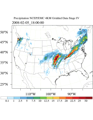
WRFDA 4D-Var can assimilate NCEP Stage IV radar and gauge precipitation data. NCEP Stage IV archived data are available on the NSF NCAR CODIAC web page (for more information, please see the NCEP Stage IV Q&A Web page). The original precipitation data are at 4-km resolution on a polar-stereographic grid. Hourly, 6-hourly, and 24-hourly analyses are available. The following image shows the accumulated 6-h precipitation for the tutorial case.
NCEP Stage IV archived data is in GRIB1 format and cannot be ingested into the WRFDA directly. The precip_converter tool is provided to reformat GRIB1 observations into the WRFDA-readable ASCII format. The NCEP GRIB libraries, w3 and g2, are required to compile the precip_converter utility. These libraries are available for download from NCEP’s GRIB2 GitHub Repository. The output file to the precip_converter utility is named in the format ob.rain.yyyymmddhh.xxh, where ‘yyyymmddhh’ is the ending hour of the accumulation period, and ‘xx’ (= 01, 06, or 24) is the accumulating time period.
Users wishing to use their own observations instead of NCEP Stage IV are responsible for writing a Fortran main program and call subroutine writerainobs (in write_rainobs.f90) to generate their own precipitation data. For more information please refer to the README file in the precip_converter directory.
Running WRFDA with Precipitation Observations
WRFDA 4D-Var is able to assimilate hourly, 3-hourly and 6-hourly precipitation data. According to experiments and related scientific papers, 6-hour precipitation accumulations are ideal, as they lead to better results than directly assimilating hourly data. The tutorial example is for assimilating 6-hour accumulated precipitation. In the working directory, link all necessary files as follows.
> ln -fs $WRFDA_DIR/var/da/da_wrfvar.exe .
> ln -fs $DAT_DIR/rc/2008020512/wrfinput_d01 .
> ln -fs $DAT_DIR/rc/2008020512/wrfbdy_d01 .
> ln -fs $DAT_DIR/rc/2008020518/wrfinput_d01 fg02
        (only necessary for var4d_lbc=true)
> ln -fs wrfinput_d01 fg
> ln -fs $DAT_DIR/be/be.dat .
> ln -fs $WRFDA_DIR/run/LANDUSE.TBL .
> ln -fs $WRFDA_DIR/run/RRTM_DATA_DBL ./RRTM_DATA
> ln -fs $DAT_DIR/ob/2008020518/ob.rain.2008020518.06h ob07.rain
        (this is explained in "Properly Linking Observation Files" below)
Edit namelist.input (start with the same namelist as for the 4dvar tutorial case) using the below guidance.
&wrfvar1 |
var4d |
true: Run WRFDA for 4DVAR. This is the only supported option for precipitation assimilation (default value is false) |
var4d_bin_rain |
length (seconds) of the precipitation assimilation window (default 3600); this can be different from var4d_bin, which controls the assimilation window for all other observation types |
&wrfvar4 |
use_rainobs |
true (default): read precipitation data |
thin_rainobs |
true (default): thin precipitation observations |
thin_mesh_conv |
size of thinning mesh (in km) for non-radiance observations, including precipitation observations (default value 20.0) |
Then, run 4D-Var in serial or parallel mode
>./da_wrfvar.exe >& wrfda.log
Properly Linking Observation Files
In the above section, ob.rain.2008020518.06h is linked as ob07.rain. The number 07 is assigned according to the following rule:
x=i*(var4d_bin_rain/var4d_bin)+1,
Here, i is the sequence number of the observation.
for x<10, the observation file should be renamed as ob0x.rain;
for x>=10, it should be renamed as obx.rain
In the example above, 6-hourly accumulated precipitation data is assimilated in a 6-hour time window. In the namelist, values should be set to
var4d_bin=3600
var4d_bin_rain=21600
There is one observation file (i.e., i=1) in the time window, thus the value of x is 7. The file ob.rain.2008020518.06h should be renamed ob07.rain.
For an example of 3-hourly precipitation data in 6-hour time window, the sample namelist is as follows.
&wrfvar1
var4d=true,
var4d_lbc=true,
var4d_bin=3600,
var4d_bin_rain=10800,
/
There are two observation files, ob.rain.2008020515.03h and ob.rain.2008020518.03h. The first file (i=1) ob.rain.2008020515.03h, is renamed ob04.rain, and the second file (i=2) is renamed ob07.rain.
Updating WRF Boundary Conditions
The ultimate goal of WRFDA is to combine a WRF file (wrfinput or wrfout) with observations and error information, in order to produce a “best guess” of the atmospheric state for the domain. While this “best guess” can be useful on its own for research purposes, it is often more useful as the initial conditions to a WRF forecast, so that the better initial conditions will ultimately provide a better forecast.
To use WRF/WRFDA for research or realtime forecast purposes, follow these steps:
Generate initial conditions for WRF (wrfinput) via WPS (as described in the WPS chapter) and real.exe (as described in the WRF Initialization chapter).
Use the generated wrfinput file from the above step to run WRFDA to assimilate observations and produce a wrfvar_output file (a new, improved wrfinput).
Run da_update_bc.exe to update the WRF lateral boundary conditions file (wrfbdy_d01) created in step 1 so that it is consistent with the new wrfinput_d01 file. Details for this process are described below in the Lateral Boundary Conditions section.
Run wrf.exe to produce a WRF forecast.
Lateral Boundary Conditions
When using a WRFDA analysis (wrfvar_output) to run a WRF forecast, it is essential to update the WRF lateral boundary conditions (contained in wrfbdy_d01, created by real.exe) to match the new WRFDA inital condition (analysis) for domain 1 to prevent discontinuities and poor results at the boundary. The update procedure is performed by the WRFDA utility da_update_bc.exe, found in $WRFDA_DIR/var/build after compiling.
da_update_bc.exe requires three input files:
the WRFDA analysis (wrfvar_output)
the wrfbdy_d01 file from real.exe
a namelist file: parame.in
To run da_update_bc.exe to update lateral boundary conditions, follow the steps below:
> cd $WRFDA_DIR/var/test/update_bc
> cp -p $DAT_DIR/rc/2008020512/wrfbdy_d01 .

*IMPORTANT: make a copy of wrfbdy_d01, as the wrf_bdy_file will be overwritten by da_update_bc.exe

> vi parame.in

&control_param
 da_file            = '../tutorial/wrfvar_output'
 wrf_bdy_file       = './wrfbdy_d01'
 domain_id          = 1
 debug              = .true.
 update_lateral_bdy = .true.
 update_low_bdy     = .false.
 update_lsm         = .false.
 iswater            = 16
 var4d_lbc          = .false.
/

> ln -sf $WRFDA_DIR/var/da/da_update_bc.exe .
> ./da_update_bc.exe
At this stage, the files wrfvar_output and wrfbdy_d01 should exist in the WRFDA working directory. They are the WRFDA updated initial and boundary condition files for any subsequent WRF model runs. To use, link a copy of wrfvar_output and wrfbdy_d01 to wrfinput_d01 and wrfbdy_d01, respectively, in the WRF working directory.
There should be two additional output files, fort.11 and fort.12, which contain information about the changes made to wrfbdy_d01.
Note
The above instructions for updating lateral boundary conditions do not apply to child domains (wrfinput_d02, wrfinput_d03, etc.). This is because the lateral boundary conditions for these domains come from the respective parent domains, so update_bc is not necessary after running WRFDA when a child domain is used as the first guess.
Cycling with WRF and WRFDA
While the above procedure is useful, often for realtime applications it is better to run a cycling forecast. In a WRF/WRFDA cycling system, rather than using WPS to generate the initial conditions for the assimilation/forecast, the output from a previous forecast is used. Information from previous observations can be used to improve the current first guess of the atmosphere, ultimately resulting in an even better analysis and forecast. The procedure for cycling is as follows:
For the initial forecast time (T1), generate initial and boundary conditions for WRF (wrfinput and wrfbdy_d01) via WPS (as described in the WPS chapter) and real.exe (as described in WRF Initialization).
Run WRFDA with this wrfinput to assimilate observations to produce a wrfvar_output file (a new, improved wrfinput).
Run da_update_bc.exe to update the WRF lateral boundary conditions file created in step 1 (wrfbdy_d01) to be consistent with the new wrfinput file.
Run wrf.exe to produce a WRF forecast (wrfout) for the next forecast time (T2).
Repeat step 1 for the next forecast time (T2) to produce initial and boundary conditions for WRF (wrfinput and wrfbdy_d01) via WPS and real.exe.
Run da_update_bc.exe to update the lower boundary conditions of the WRF forecast file (wrfout) with data from the wrfinput file generated in step 5.
Run WRFDA using this wrfout file to assimilate observations and produce a wrfvar_output file (a new, improved wrfinput for the next WRF forecast).
Run da_update_bc.exe again to update the WRF boundary conditions file created in step 5 (wrfbdy_d01) so they are consistent with the new wrfinput file.
Run wrf.exe to produce a WRF forecast (wrfout) for the next forecast time (T2).
Repeat steps 5-9 for the next forecast time(s) ad infinitum (T3, T4, T5, …).
In cycling mode, da_update_bc.exe is used for two distinct purposes:
Prior to running WRFDA, it updates the lower boundary conditions for the WRF forecast file that is used as the first guess for WRFDA, then after running WRFDA, it updates the lateral boundary conditions file (wrfbdy_d01) so that it is consistent with the WRFDA output (a new, improved wrfinput for the next WRF forecast) - this purpose was discussed in the previous section
To update the lower boundary conditions - discussed in this section
While a WRF forecast integrates atmospheric variables forward in time, it does not update certain lower boundary conditions, such as vegetation fraction, sea ice, snow cover, etc., which are important for both forecasts and data assimilation. For short periods of time, this is not a problem, as these fields do not tend to evolve much over the course of a few days. However, for a cycling forecast that runs for weeks, months, or even years, it is essential to update these fields regularly from the initial condition files through WPS.
To do this, prior to the assimilation process, the first guess file needs to be updated based on the information from the wrfinput file, generated by WPS/real.exe at analysis time. Run da_update_bc.exe with the following namelist options.
da_file            = './fg'
wrf_input          = './wrfinput_d01'
update_lateral_bdy = .false.
update_low_bdy     = .true.
iswater            = 16
Note
‘iswater’ (water point index) is 16 for USGS LANDUSE and 17 for MODIS LANDUSE.
This creates a lower-boundary updated first guess (da_file is overwritten by da_update_bc with updated lower boundary conditions from wrf_input). After WRFDA has finished, run da_update_bc.exe again with the following namelist options:
da_file            = './wrfvar_output'
wrf_bdy_file       = './wrfbdy_d01'
update_lateral_bdy = .true.
update_low_bdy     = .false.
This updates the lateral boundary conditions (wrf_bdy_file is overwritten by da_update_bc with lateral boundary conditions from da_file).
Lateral boundary conditions for child domains (wrfinput_d02, wrfinput_d03, etc.) come from the respective parent domains, so update_bc is not necessary after running WRFDA. However, for cycling, the lower boundaries in each nested domain’s WRFDA analysis file still need to be updated. The namelist variable, domain_id should be set > 1 (default is 1 for domain 1) and provide the appropriate wrfinput file (e.g., wrf_input = ‘./wrfinput_d02’ for domain 2).
WRFDA 4DVAR with Lateral Boundary Conditions as Control Variables
If var4d_lbc is activated in a WRF 4D-Var run, in addition to the above-mentioned files, the ana02 file from the WRFDA working directory is needed. In parame.in, set var4d_lbc to .true. and use da_file_02 to point to the location of the ana02 file.
da_file_02         = './ana02'
var4d_lbc          = .true.
Background Error (BE) and Running GEN_BE
Quick-start Guide: Running WRFDA with Different BE Options
To run WRFDA with the generic CV3 option, simply link the provided be.dat file in the var/run directory:
> cp -p $WRFDA_DIR/var/run/be.dat.cv3 $WORK_DIR/be.dat
To run WRFDA with any other option, GEN_BE must be run first. GEN_BE takes a series of forecasts initialized at different times, and compares forecasts that are valid at the same time (e.g., compare a 24-hour forecast initialized at 00Z with a 12-hour forecast initialized at 12Z) to get an estimate of the background error statistics.
The wrapper script gen_be_wrapper.ksh is used to run GEN_BE. For instructions on how to set up experiments to run GEN_BE, reference the test case as described in Domain-specific background error options: Running GEN_BE below.
Background Error Options in WRFDA
Users have four choices to define the background error covariance (BE): CV3, CV5, CV6, and CV7. Each of these has different properties, which are outlined in the table below:
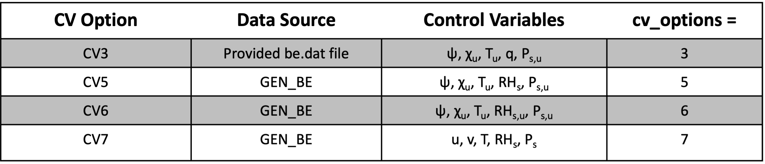
The primary differences between CV3 and the remaining BEs (CV5, CV6, and CV7) are: CV3
control variables are in physical space
uses the vertical recursive filter to model vertical covariance
this is a global BE that can be used for any regional domain
- CV5, CV6, CV7
control variables are in eigenvector space
use an empirical orthogonal function (EOF) to represent vertical covariance
domain-dependent - should be generated based on forecast or ensemble data from the same domain
As summarized in the above table, CV5, CV6, and CV7 differ in the control variables they use. CV5 utilizes streamfunction (Ψ), unbalanced velocity potential (Χu), unbalanced temperature (Tu), pseudo relative humidity (RHs), and unbalanced surface pressure (Ps,u). The pseudo relative humidity is defined as Q/Qb,s, where Qb,s is the saturated specific humidity from the background field. For CV6 the moisture control variable is the unbalanced portion of the pseudo relative humidity (RHs,u). Additionally, CV6 introduces six additional correlation coefficients in the definition of the balanced part of analysis control variables. See the section GEN_BE for CV6 for more details on this option. Finally, CV7 uses a different set of control variables: u, v, temperature, pseudo relative humidity (RHs), and surface pressure (Ps).
test
Generic BE Option: CV3
CV3 is the NCEP background error covariance. It is estimated in grid space by what has become known as the NMC method (Parrish and Derber 1992) . The statistics are estimated with the differences of 24 and 48-hour GFS forecasts with T170 resolution, valid at the same time for 357 cases, distributed over a period of one year. Both the amplitudes and the scales of the background error have to be tuned to represent the forecast error in the estimated fields. The statistics that project multivariate relations among variables are also derived from the NMC method.
The variance of each variable, and the variance of its second derivative, are used to estimate its horizontal scales. For example, the horizontal scales of the stream function can be estimated from the variance of the vorticity and stream function.
The vertical scales are estimated with the vertical correlation of each variable. A table is built to cover the range of vertical scales for the variables. The table is then used to find the scales in vertical grid units. The filter profile and the vertical correlation are fitted locally. The scale of the best fit from the table is assigned as the scale of the variable at that vertical level for each latitude. Note that the vertical scales are locally defined so that the negative correlation further away, in the vertical direction, is not included.
Theoretically, CV3 BE is a generic background error statistics file which can be used for any case. It is quite straightforward to use CV3 in your own case. To use the CV3 BE file in your case, set cv_options=3 in &wrfvar7 in namelist.input in your working directory, and use the be.dat is located in WRFDA/var/run/be.dat.cv3.
Modifying CV3 Length Scales and Variance
Because CV3 is a generic background error option, it is necessary to tune the default background error scale length and variance values for each experiment. These can be controlled at run time with a series of namelist variables described below.
The scaling factors for CV3 are stored as an array of values for each individual control variable:
as1: stream function
as2: unbalanced velocity potential
as3: unbalanced temperature
as4: pseudo relative humidity
as5: unbalanced surface pressure
These variables are all 3-element vectors. The first element is the variance scaling factor. The second is the horizontal length scale factor. The third is the vertical length scale factor. So setting the default values in your namelist would look like this:
&wrfvar7
  cv_options = 3,
  as1     =  0.25,   1.00,   1.50,
  as2     =  0.25,   1.00,   1.50,
  as3     =  0.25,   1.00,   1.50,
  as4     =  0.25,   1.00,   1.50,
  as5     =  0.25,   1.00,   1.50,
 /
The first column is the variance, the second is the horizontal length scale factor, and the third is the vertical length scale factor.
For multiple outer loops, the next 3 elements of each vector must be filled in. So for 2 outer loops (max_ext_its=2), to use the default values, the namelist should look like this:
&wrfvar7
  cv_options = 3,
  as1     =  0.25,   1.00,   1.50,   0.25,   1.00,   1.50,
  as2     =  0.25,   1.00,   1.50,   0.25,   1.00,   1.50,
  as3     =  0.25,   1.00,   1.50,   0.25,   1.00,   1.50,
  as4     =  0.25,   1.00,   1.50,   0.25,   1.00,   1.50,
  as5     =  0.25,   1.00,   1.50,   0.25,   1.00,   1.50,
 /
Again, the first column is the variance, the second is the horizontal length scale factor, and the third is the vertical length scale factor for the first outer loop. The fourth column is the variance, the fifth is the horizontal length scale factor, and the sixth is the vertical length scale factor for the second outer loop.
Continue in this manner for more outer loops. The values listed above are the default values, but can be adjusted for each individual experiment.
Domain-specific Background Error Options: Running GEN_BE
To use CV5, CV6 or CV7 background error covariance, it is necessary to generate your domain-specific background error statistics with the gen_be utility. The default CV3 background error statistics file, supplied with the WRFDA source code, can NOT be used with these control variable options.
The main source code for the various gen_be stages can be found in WRFDA/var/gen_be. The executables of gen_be should have been created when you compiled the WRFDA code (as described earlier). The scripts to run these codes are in WRFDA/var/scripts/gen_be. The user can run gen_be using the wrapper script WRFDA/var/scripts/gen_be/gen_be_wrapper.ksh.
The input data for gen_be are WRF forecasts, which are used to generate model perturbations, used as a proxy for estimates of forecast error. For the NMC-method, the model perturbations are differences between forecasts (e.g. T+24 minus T+12 is typical for regional applications, T+48 minus T+24 for global) valid at the same time. Climatological estimates of background error may then be obtained by averaging these forecast differences over a period of time (e.g. one month). Given input from an ensemble prediction system (EPS), the inputs are the ensemble forecasts, and the model perturbations created are the transformed ensemble perturbations. The gen_be code has been designed to work with either forecast difference or ensemble-based perturbations. The former is illustrated in this tutorial example.
It is important to include forecast differences valid at different parts of the day (for example, forecasts valid at 00Z and 12Z through the forecast period) to remove contributions from the diurnal cycle (i.e. do not run gen_be using model perturbations valid for a single time each day).
The inputs to gen_be are netCDF WRF forecast output (“wrfout”) files at specified forecast ranges. To avoid unnecessary large single data files, it is assumed that all forecast ranges are output to separate files. For example, if we wish to calculate BE statistics using the NMC-method with (T+24)-(T+12) forecast differences (default for regional) then by setting the WRF namelist.input options history_interval=720, and frames_per_outfile=1 we get the necessary output data sets. Then the forecast output files should be arranged as follows: directory name is the forecast initial time, time info in the file name is the forecast valid time. 2008020512/wrfout_d01_2008-02-06_00:00:00 means a 12-hour forecast valid at 2008020600, initialized at 2008020512.
An example tutorial case data set for a test case (90 x 60 x 41 gridpoints) can be downloaded. Untar the gen_be_forecasts_20080205.tar.gz file. You will have:
>ls $FC_DIR

-rw-r--r--  1   users  11556492 2008020512/wrfout_d01_2008-02-06_00:00:00
-rw-r--r--  1   users  11556492 2008020512/wrfout_d01_2008-02-06_12:00:00
-rw-r--r--  1   users  11556492 2008020600/wrfout_d01_2008-02-06_12:00:00
-rw-r--r--  1   users  11556492 2008020600/wrfout_d01_2008-02-07_00:00:00
-rw-r--r--  1   users  11556492 2008020612/wrfout_d01_2008-02-07_00:00:00
-rw-r--r--  1   users  11556492 2008020612/wrfout_d01_2008-02-07_12:00:00
In the above example, only 1 day (12Z 05 Feb to 12Z 06 Feb. 2008) of forecasts, every 12 hours is supplied to gen_be_wrapper to estimate forecast error covariance. It is only for demonstration. The minimum number of forecasts required depends on the application, number of grid points, etc. Month-long (or longer) data sets are typical for the NMC-method. Generally, at least a 1-month data set should be used.
Under WRFDA/var/scripts/gen_be, gen_be_wrapper.ksh is used to generate the BE data. The following variables need to be set to fit your case:
export WRFVAR_DIR=/glade/work/wrfhelp/PRE_COMPILED_CODE/WRFDA
export NL_CV_OPTIONS=5        # 5 for CV5, 7 for CV7
export START_DATE=2008020612  # the first perturbation valid date
export END_DATE=2008020700    # the last perturbation valid date
export NUM_LEVELS=40          # e_vert - 1
export BIN_TYPE=5             # How data is binned for calculating statistics
export FC_DIR=/glade/work/wrfhelp/WRFDA_DATA/fc   # where wrf forecasts are
export RUN_DIR=`pwd`/gen_be   # Where GEN_BE will run and output files
Note
The START_DATE and END_DATE are perturbation valid dates. As shown in the forecast list above, when you have 24-hour and 12-hour forecasts initialized at 2008020512, through 2008020612, the first and final forecast difference valid dates are 2008020612 and 2008020700, respectively.
The forecast data set should be located in $FC_DIR. Then type:
> gen_be_wrapper.ksh
Once the gen_be_wrapper.ksh run is completed, the be.dat can be found under the $RUN_DIR directory. To get a clear idea about what is included in be.dat, the script gen_be_plot_wrapper.ksh may be used. This plots various data in be.dat; for example:
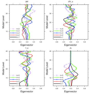
GEN_BE for CV6
CV6 is a multivariate background error statistics option in WRFDA. It may be activated by setting the namelist variable cv_options=6. This option introduces six additional correlation coefficients in the definition of the balanced part of analysis control variables. Thus with this implementation, moisture analysis is multivariate, in the sense that temperature and wind may lead to moisture increments, and vice-versa. Further details are available in Implementation of multivariate background error (MBE) statistics in WRFDA.
How to generate CV6 background error statistics for WRFDA
CV6 background error statistics for WRFDA are generated by executing a top-level script, gen_be/wrapper_gen_mbe.ksh, residing under SCRIPTS_DIR via a suitable wrapper script. The rest of the procedure remains the same as with normal running of the gen_be utility. A successful run will create a be.dat file in the RUN_DIR directory.
How to run WRFDA with CV6 background error statistics
After successfully generating the CV6 background error statistics file be.dat, the procedure for running WRFDA is straight-forward: Include cv_options=6 in the namelist.input file under the &wrfvar7 list of namelist options.
How to tune CV6 background error statistics
Below is a list of nine tuning parameters available in WRFDA; these can be specified under &wrfvar7 in the namelist. Default values for these variables are set as 1.0. Setting corresponding values > 1.0 (< 1.0) will increase (decrease) the corresponding contributions:
Variable Name |
Description |
|---|---|
psi_chi_factor |
Parameter to control contribution of stream function in defining balanced part of velocity potential |
psi_t_factor |
Parameter to control contribution of stream function in defining balanced part of temperature |
psi_ps_factor |
Parameter to control contribution of stream function in defining balanced part of surface pressure |
psi_rh_factor |
Parameter to control contribution of stream function in defining balanced part of moisture |
chi_u_t_factor |
Parameter to control contribution of unbalanced part of velocity potential in defining balanced part of temperature |
chi_u_ps_factor |
Parameter to control contribution of unbalanced part of velocity potential in defining balanced part of surface pressure |
chi_u_rh_factor |
Parameter to control contribution of unbalanced part of velocity potential in defining balanced part of moisture |
t_u_rh_factor |
Parameter to control contribution of unbalanced part of temperature in defining balanced part of moisture |
ps_u_rh_factor |
Parameter to control contribution of unbalanced part of surface pressure in defining balanced part of moisture |
Additional Background Error Options
Single Observation Response in WRFDA
With the single observation test, you may get some ideas of how the background and observation error statistics work in the model variable space. A single observation test is done in WRFDA by setting num_pseudo=1, along with other pre-specified values in record &wrfvar15 and &wrfvar19 of namelist.input.
With the settings shown below, WRFDA generates a single observation with a pre-specified innovation (Observation - First Guess) value at the desired location; e.g. at (in terms of grid coordinate) 23x23, level 14 for U observation with error characteristics 1 m/s, and innovation size = 1.0 m/s.
&wrfvar15
num_pseudo = 1,
pseudo_x = 23.0,
pseudo_y = 23.0,
pseudo_z = 14.0,
pseudo_err = 1.0,
pseudo_val = 1.0,
/

&wrfvar19
pseudo_var = 'u',
/
You may wish to repeat this exercise for other observation types. pseudo_var can take any of the following values:
Variable Name |
Description |
Units |
|---|---|---|
u |
East-west wind |
m/s |
v |
North-south wind |
m/s |
t |
Temperature |
K |
p |
Pressure |
Pa |
q |
Water vapor mixing ratio |
unitless (kg/kg) |
qcw |
Water vapor mixing ratio |
unitless (kg/kg) |
qrn |
Rain water mixing ratio |
unitless (kg/kg) |
qci |
Cloud ice mixing ratio |
unitless (kg/kg) |
qsn |
Snow mixing ratio |
unitless (kg/kg) |
qgr |
Graupel mixing ratio |
unitless (kg/kg) |
tpw |
Total precipitable water |
cm |
ztd |
GPS zenith total delay |
cm |
ref |
GPS Refractivity |
Unitless |
Response of BE Length Scaling Parameter
Run the single observation test with the following additional parameters in record &wrfvar7 of namelist.input.
&wrfvar7
len_scaling1 = 0.5, # reduce psi length scale by 50%
len_scaling2 = 0.5, # reduce chi_u length scale by 50%
len_scaling3 = 0.5, # reduce T length scale by 50%
len_scaling4 = 0.5, # reduce q length scale by 50%
len_scaling5 = 0.5, # reduce Ps length scale by 50%
/
Note
You may wish to try the response of an individual variable by setting one parameter at a time. Note the spread of analysis increment.
Response of Changing BE Variance
Run the single observation test with the following additional parameters in record &wrfvar7 of namelist.input.
&wrfvar7
var_scaling1 = 0.25,   # reduce psi variance by 75%
var_scaling2 = 0.25,   # reduce chi_u variance by 75%
var_scaling3 = 0.25,   # reduce T variance by 75%
var_scaling4 = 0.25,   # reduce q variance by 75%
var_scaling5 = 0.25,   # reduce Ps variance by 75%
/
Note
You may wish to try the response of individual variable by setting one parameter at a time. Note the magnitude of analysis increments.
WRFDA Diagnostics
WRFDA produces a number of diagnostic files that contain useful information on how the data assimilation has performed. This section will introduce you to some of these files, and what to look for.
After running WRFDA, it is important to check a number of output files to see if the assimilation appears sensible. The WRFDA package, which includes several useful scripts, may be downloaded from the WRFDA Tools Package.
The content of some useful diagnostic files are as follows:
cost_fn and grad_fn: These files hold (in ASCII format) WRFDA cost and gradient function values, respectively, for the first and last iterations.
If you run with calculate_cg_cost_fn=true and write_detail_grad_fn=true, however, these values will be listed for each iteration; this can be helpful for visualization purposes.
The NCL script in the WRFDA TOOLS package located at var/graphics/ncl/plot_cost_grad_fn.ncl may be used to plot the content of cost_fn and grad_fn, if these files are generated with calculate_cg_cost_fn=true and write_detail_grad_fn=true.
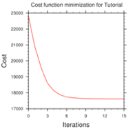
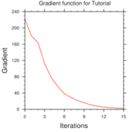
Note
Make sure that you remove the first two lines (header) in cost_fn and grad_fn before you plot. You also need to specify the directory name for these two files.
gts_omb_oma_01 : It contains (in ASCII format) information on all of the observations used by the WRFDA run. Each observation has its observed value, quality flag, observation error, observation minus background (OMB), and observation minus analysis (OMA). This information is very useful for both analysis and forecast verification purposes.
namelist.input : This is the WRFDA input namelist file, which contains all the user-defined non-default options. Any namelist-defined options that do not appear in this file should have their names checked against the values in $WRFDA_DIR/Registry/registry.var.
namelist.output.da : A list of all the namelist options used. If an option was not specified in namelist.input, the default listed in the registry value will be used.
rsl : Files containing information for standard WRFDA output from individual processors when multiple processors are used. It contains a host of information on a number of observations, minimization, timings, etc. Additional diagnostics may be printed in these files by including various print WRFDA namelist options. To learn more about these additional print options, search for the print_ string in $WRFDA_DIR/Registry/registry.var.
statistics : Text file containing OMB (OI) and OMA (OA) statistics (minimum, maximum, mean and standard deviation) for each observation type and variable. This information is very useful in diagnosing how WRFDA has used different components of the observing system. Also contained are the analysis minus background (A-B) statistics, i.e. statistics of the analysis increments for each model variable at each model level. This information is very useful in checking the range of analysis increment values found in the analysis, and where they are in the WRF-model grid space.
The WRFDA analysis file is wrfvar_output. It is in WRF (netCDF) format. It will become the input file wrfinput_d01 of any subsequent WRF run after lateral boundary and/or lower boundary conditions are updated by another WRFDA utility (See the section Updating WRF Boundary Conditions).
An NCL script, $TOOLS_DIR/var/graphics/ncl/WRF-Var_plot.ncl, is provided in the tools package for plotting. You need to specify the analysis_file name, its full path, etc. Please see the in-line comments in the script for details.
As an example, if you are aiming to display the U-component of the analysis at level 18, use the script WRF-Var_plot.ncl, and make sure the following pieces of codes are uncommented:
var = "U"
fg = first_guess->U
an = analysis->U
plot_data = an
When you execute the following command from $WRFDA_DIR/var/graphics/ncl.
> ncl WRF-Var_plot.ncl
The plot should look like:
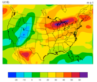
You may change the variable name, level, etc. in this script to display the variable of your choice at the desired eta level. Take time to look through the text output files to ensure you understand how WRFDA works. For example:
How closely has WRFDA fit individual observation types? Look at the statistics file to compare the O-B and O-A statistics.
How big are the analysis increments? Again, look in the statistics file to see minimum/maximum values of A-B for each variable at various levels. It will give you a feel for the impact of the input observation data you assimilated via WRFDA by modifying the input analysis first guess.
How long did WRFDA take to converge? Does it really converge? You will get the answers of all these questions by looking into the rsl.* -files, as it indicates the number of iterations taken by WRFDA to converge. If this is the same as the maximum number of iterations specified in the namelist (NTMAX), or its default value (=200) set in $WRFDA_DIR/Registry/registry.var, then it means that the analysis solution did not converge. If this is the case, you may need to increase the value of NTMAX and rerun your case to ensure that the convergence is achieved. On the other hand, a normal WRFDA run should usually converge within 100 iterations. If it still does not converge in 200 iterations, that means there may be a problem in the observations or first guess.
A good way to visualize the impact of assimilation of observations is to plot the analysis increments (i.e. analysis minus the first guess difference). Many different graphics packages (e.g. RIP4, NCL, GRADS etc) can do this.
You need to modify this script to fix the full path for first_guess and analysis files. You may also use it to modify the display level by setting kl and the name of the variable to display by setting var. Further details are given in this script.
If you are aiming to display the increment of potential temperature at level 18, after modifying $WRFDA_DIR/var/graphics/ncl/WRF-Var_plot.ncl, make sure the following pieces of code are uncommented:
var = "T"
fg = first_guess->T ;Theta- 300
an = analysis->T    ;Theta- 300
plot_data = an - fg
When you execute the following command from WRFDA_DIR/var/graphics/ncl.
> ncl WRF-Var_plot.ncl
The plot created will look as follows:
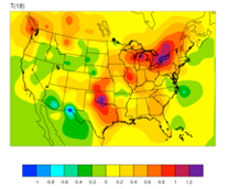
Note
Larger analysis increments indicate a larger data impact in the corresponding region of the domain.
Generating Ensembles with RANDOMCV
In addition to the variational methods previously mentioned, the WRFDA system supports both ensemble and hybrid ensemble/variational assimilation methods. To utilize these methods, having an ensemble of forecasts is necessary. WRFDA has a built-in method for generating ensemble initial conditions known as RANDOMCV. RANDOMCV works by adding random noise to the analysis in control variable space.
Running WRFDA for RANDOMCV
RANDOMCV is a capability of the main WRFDA executable, so you will run it by setting the following variables in namelist.input and then running da_wrfvar.exe as you would with any data assimilation run:
&wrfvar5 |
put_rand_seed |
true : enter your own seed numbers to generate random background perturbations; the advantage of this setting is that the same seed numbers will always produce the same perturbation |
&wrfvar11 |
seed_array1 |
First integer for seeding the random function (default: 1) |
seed_array2 |
Second integer for seeding the random function (default: 1); it is not necessary to change both seeds to get different perturbations |
&wrfvar17 |
analysis_type |
Set this to RANDOMCV to use the RANDOMCV capability |
n_randomcv |
1 (default); number of ensemble to be generated in one run; new in version 4.2 |
When setting your own random seeds, a common good practice is to set the first seed as the experiment date/time in integer form, and the second seed as the ensemble member number. The seeds should not be set to zero.
Because the perturbations are made in control variable space, the general pattern of perturbations will depend on your background error. You should be able to use any background error option with RANDOMCV (CV3, CV5, CV6, or CV7). Additionally, this means you can control their magnitude and lengthscales by modifying the background error variance and length scaling variables respectively:
For CV5, CV6, or CV7
&wrfvar7
var_scaling1 = 0.25,  # reduce psi perturbation magnitude by 75%
var_scaling2 = 0.25,  # reduce chi_u perturbation magnitude by 75%
var_scaling3 = 0.0,   # reduce T perturbation by 100% (there will be no T perturbation!)
var_scaling4 = 2.0,   # increase q perturbation by 100%
var_scaling5 = 1.0,   # Keep Ps perturbation magnitude the same
len_scaling1 = 0.5,   # reduce psi perturbation length scale by 50%
len_scaling2 = 0.5,   # reduce chi_u perturbation length scale by 50%
len_scaling3 = 1.0,   # Keep T perturbation length scale the same
len_scaling4 = 2.0,   # increase q perturbation length scale by 100%
len_scaling5 = 1.5,   # increase Ps perturbation length scale by 50%
/
For CV3
See Modifying CV3 Length Scales and Variance in the Generic BE Option: CV3 section.
Hybrid Data Assimilation in WRFDA
The WRFDA system also includes hybrid data assimilation techniques - both 3DEnVar and 4DEnVar, which is based on the previously-described variational capability.
The difference between hybrid and variational schemes is that WRFDA 3DVAR and 4DVAR rely solely on a static covariance model to specify the background errors, while the hybrid system uses a combination of static error covariances and ensemble-estimated error covariances to incorporate a flow-dependent estimate of the background error statistics. The following sections will give a brief introduction to using the hybrid system. Please refer to these papers for a detailed description of the methodology used in the WRFDA hybrid system:
Four executables are used in the hybrid system. If you have successfully compiled the WRFDA system, the following executables will exist in the WRFDA/var/build directory:
WRFDA/var/build/gen_be_ensmean.exe
WRFDA/var/build/gen_be_ep2.exe
WRFDA/var/build/da_wrfvar.exe
WRFDA/var/build/gen_be_vertloc.exe
gen_be_ensmean.exe is used to calculate the ensemble mean, while gen_be_ep2.exe is used to calculate the ensemble perturbations. gen_be_vertloc.exe is used for vertical localization. As with 3DVAR/4DVAR, da_wrfvar.exe is the main WRFDA program. However, in this case, da_wrfvar.exe will run in hybrid mode.
Running the Hybrid System for 3DEnVar
The procedure is the same as running 3DVAR, with the exception of some extra input files and namelist settings. The basic input files for WRFDA are LANDUSE.TBL, ob.ascii or ob.bufr (depending on which observation format you use), and be.dat (static background errors). Additional input files required for 3DEnVar are a single ensemble mean file (used as the fg for the hybrid application) and a set of ensemble perturbation files (used to represent flow-dependent background errors).
A set of initial ensemble members must be prepared before the hybrid application can be started. The ensemble can be obtained from other ensemble model outputs, or you can generate them yourself. This can be done, for example, adding random noise to the initial conditions at a previous time and integrating each member to the desired time (download a 3DEnVar tutorial case with a test ensemble). In this example, the ensemble forecasts were initialized at 2015102612 and valid 2015102712. A hybrid analysis at 2015102712 will be performed using the ensemble valid 2015102712 as input. Once you have the initial ensemble, the ensemble mean and perturbations can be calculated following the steps below:
Set an environment variable for your working directory and your data directory
> setenv WORK_DIR your_hybrid_path
> setenv DAT_DIR your_data_path
> cd $WORK_DIR
Calculate the ensemble mean
From your working directory, copy or link the ensemble forecasts to your working directory. The ensemble members are identified by the characters .e### at the end of the file name, where ### represents three-digit numbers following the valid time.
> ln -sf $DAT_DIR/Hybrid/fc/2015102612/wrfout_d01_2015-10-27_12:00:00.e* .Provide two template files (ensemble mean and variance files) in your working directory. These files will be overwritten with the ensemble mean and variance as discussed below.
> cp $DAT_DIR/Hybrid/fc/2015102612/wrfout_d01_2015-10-27_12:00:00.e001 ./wrfout_d01_2015-10-27_12:00:00.mean
> cp $DAT_DIR/Hybrid/fc/2015102612/wrfout_d01_2015-10-27_12:00:00.e001 ./wrfout_d01_2015-10-27_12:00:00.vari
Copy gen_be_ensmean_nl.nl (cp $DAT_DIR/Hybrid/gen_be_ensmean_nl.nl .) You will need to set the information in this script as follows:
&gen_be_ensmean_nl
directory = '.'
filename = 'wrfout_d01_2015-10-27_12:00:00'
num_members = 10
nv = 7
cv = 'U', 'V', 'W', 'PH', 'T', 'MU', 'QVAPOR'
/
where directory is the folder containing the ensemble members and template files, filename is the name of the files before their suffixes (e.g., .mean, .vari, etc), num_members is the number of ensemble members you are using, nv is the number of variables, and cv is the name of variables used in the hybrid system. Be sure nv and cv are consistent!
Link gen_be_ensmean.exe to your working directory and run it.
> ln -sf  $WRFDA_DIR/var/build/gen_be_ensmean.exe .
> ./gen_be_ensmean.exe
Check the output files. wrfout_d01_2015-10-27_12:00:00.mean is the ensemble mean; wrfout_d01_2015-10-27_12:00:00.vari is the ensemble variance
Calculate ensemble perturbations
Create a sub-directory in which you will be working to create ensemble perturbations.
> mkdir -p ./ep
> cd ./ep
Run gen_be_ep2.exe. The executable requires four command-line arguments (DATE, NUM_MEMBER, DIRECTORY, and FILENAME) as shown below for the tutorial example:
> ln -sf $WRFDA_DIR/var/build/gen_be_ep2.exe  .
> ./gen_be_ep2.exe  2015102712  10  .  ../wrfout_d01_2015-10-27_12:00:00
Check the output files. A list of binary files should now exist. Among them, tmp.e* are temporary scratch files that can be removed.
Back in the working directory, create the input file for vertical localization. This program requires one command-line argument: the number of vertical levels of the model configuration (same value as e_vert in the namelist; for the tutorial example, this should be 42).
> cd $WORK_DIR
> ln -sf $WRFDA_DIR/var/build/gen_be_vertloc.exe .
> ./gen_be_vertloc.exe 42
The output is ./be.vertloc.dat in your working directory.
Run WRFDA in hybrid mode
In your hybrid working directory, link all the necessary files and directories as follows:
> ln -fs ./wrfout_d01_2015-10-27_12:00:00.mean ./fg  (first guess is the ensemble mean for this test case)
> ln -fs $WRFDA_DIR/run/LANDUSE.TBL .
> ln -fs $DAT_DIR/Hybrid/ob/2015102712/ob.ascii ./ob.ascii
> ln -fs $DAT_DIR/Hybrid/be/be.dat ./be.dat
> ln -fs $WRFDA_DIR/var/build/da_wrfvar.exe .
> cp $DAT_DIR/Hybrid/namelist.input .
Edit namelist.input, paying special attention to the following hybrid-related settings:
&wrfvar7
je_factor = 2.0
/

&wrfvar16
ensdim_alpha = 10
alphacv_method = 2
alpha_corr_type=3
alpha_corr_scale = 500.0
alpha_std_dev=1.000
alpha_vertloc_opt = 2
ep_format = 1
/
Finally, execute the WRFDA file, running in hybrid mode
> ./da_wrfvar.exe >& wrfda.logCheck the output files; the output file lists are the same as when you run WRF 3D-Var.
Running the Hybrid System for 4DEnVar
The procedure for 4DEnVar is very similar to the procedure for 3DEnVar. Unlike 4DVAR, 4DEnVar does not require WRFPLUS, the tangent linear/adjoint model. It is more analogous to the First Guess at Appropriate Time (FGAT) method than full 4DVAR. Like FGAT, 4DEnVar requires multiple first guess files, one for each assimilation time window. In addition, you must have ensemble output for each of the first guess times, and generate ensemble perturbations from each of these sets of ensemble forecasts.
To activate the 4DEnVar option, set the namelist variable use_4denvar=.true. under &wrfvar16 (download a 4DEnVar tutorial case with a test ensemble). In this example, the ensemble forecasts were initialized at 2005071512 and valid for 2005071521 - 2005071603. The 4DEnVar hybrid analysis (wrfvar_output) will be valid for 2005071600.
Dual-resolution Hybrid
WRFDA has an option for dual-resolution hybrid data assimilation, where a high-resolution background can make use of a lower-resolution ensemble for extracting the flow-dependent contribution to the background error. The lower-resolution ensemble should be the parent domain of the higher-resolution child domain that the analysis is performed on.
Performing dual-resolution hybrid assimilation is similar to the process for regular assimilation described above. The main difference is that you must include some settings in the &domains section of the namelist in a different way: The setting max_dom=2 must be used, and for each column of settings, the low-resolution domain settings must be listed first, even though the second column will be the domain on which assimilation is being performed. An example of the &domains namelist section is shown below; in this case, the low-resolution ensemble domain is 222x128 grid points at 45 km resolution, and the high-resolution analysis domain is 184x196 grid points at 15 km resolution:
&domains
 time_step            = 90,
 max_dom              = 2,
 s_we                 =   1,   1,
 e_we                 = 222, 184,
 s_sn                 =   1,   1,
 e_sn                 = 128, 196,
 s_vert               =   1,   1,
 e_vert               =  45,  45,
 dx                   = 45000, 15000,
 dy                   = 45000, 15000,
 grid_id              = 1,  2,
 parent_id            = 0,  1,
 i_parent_start       = 0, 89,
 j_parent_start       = 0, 22,
 parent_grid_ratio    = 1,  3,
/
For further details about any of the above settings, see the Namelist Variables chapter of this Users’ Guide.
In addition to the above, you must set the namelist variable hybrid_dual_res=true, as well as providing a file named fg_ens in the working directory. This file can be any WRF input or wrfout file that has the same domain as the low-resolution ensemble; it is merely used for reading in mapping parameters for the low-resolution ensemble domain.
The dual-resolution hybrid capability is described in more detail in Sensitivity of Limited-area Hybrid Variational-ensemble Analyses and Forecasts to Ensemble Perturbation Resolutions
Hybrid Namelist Options
&wrfvar7 |
je_factor |
ensemble covariance weighting factor; this factor controls the weighting component of ensemble and static covariances; the corresponding jb_factor = je_factor/(je_factor - 1) |
&wrfvar16 |
use_4denvar |
.true. will activate 4DEnVar |
hybrid_dual_res |
.true. will activate dual-resolution mode |
ep_para_read |
Method for reading ensemble perturbation files |
rden_bin |
bins for parallel reading of ensemble perturbation files; default is 1; lower numbers use more memory, but are faster; if memory use becomes too large, increase this value |
ensdim_alpha |
the number of ensemble members; hybrid mode is activated when ensdim_alpha is larger than zero |
alphacv_method |
2 (default): perturbations in model space (u, v, t, q, ps); option 2 is extensively tested and recommended to use |
alpha_corr_type |
correlation function |
alpha_corr_scale |
hybrid covariance localization scale in km unit; default value is 200 |
alpha_std_dev |
alpha standard deviation; default value is 1.0 |
alpha_vertloc_opt |
(new in version 4.2) |
ep_format |
(new in version 4.2) |
ETKF Data Assimilation
The WRFDA system also includes a ETKF assimilation technique. The ETKF system updates the ensemble perturbations. Please refer to Bishop et al. (2001) and Wang et al. (2003) for a detailed description of the methodology. The following section will give a brief introduction of some aspects of using the ETKF system.
Source Code
Three executables are used in the ETKF system. If you have successfully compiled the WRFDA system, you will see the following:
WRFDA/var/build/gen_be_etkf.exe
WRFDA/var/build/gen_be_addmean.exe
WRFDA/var/build/da_wrfvar.exe
The file gen_be_etkf.exe is used to update the ensemble perturbations, while gen_be_addmean.exe is used to combine the ensemble mean and the ensemble perturbations. As with 3D-Var/4D-Var, da_wrfvar.exe is the main WRFDA program. However, in this case, da_wrfvar.exe will create filtered observations and prepare formatted omb files for ETKF.
Running the ETKF System
The first procedure is to update the ensemble perturbations. A set of initial ensemble members must be prepared before the ETKF application can be started. The ensemble can be obtained from a previous ensemble forecast (download an ETKF tutorial case with a test ensemble). In this example, the ensemble forecasts were initialized at 2015102612 and valid 2015102712. ETKF will be performed using the ensemble valid 2015102712 as input. Once you have the initial ensemble, the ensemble perturbations can be updated by following the steps below:
Set environment variables for convenience
> setenv WORK_DIR_ETKF your_etkf_path
> setenv DAT_DIR your_data_path
> setenv WRFDA_DIR your_WRFDA_path
> cd $WORK_DIR_ETKF
Prepare the filtered observations
In your ETKF working directory, make a subdirectory to prepare the filtered observations and link all the necessary files and directories as follows:
> mkdir obs_filter
> cd obs_filter
> ln -fs $DAT_DIR/Hybrid/fc/2015102612/wrfout_d01_2015-10-27_12:00:00.mean ./fg
        (first guess is the ensemble mean)
> ln -fs $WRFDA_DIR/run/LANDUSE.TBL .
> ln -fs $DAT_DIR/Hybrid/ob/2015102712/ob.ascii ./ob.ascii
> ln -fs $DAT_DIR/Hybrid/be/be.dat ./be.dat
> ln -fs $WRFDA_DIR/var/build/da_wrfvar.exe .
> cp $DAT_DIR/ETKF/namelist.input .
Edit namelist.input, paying special attention to the following ‘QC-OBS’-related settings:
&wrfvar17
 analysis_type = 'QC-OBS',
/
Execute the WRFDA file, running in QC-OBS mode
> ./da_wrfvar.exe >& wrfda.logCheck the output files; you should see a ‘filtered_obs_01’ file which contains the filtered observations.
Prepare omb files for ETKF
In your ETKF working directory, make a subdirectory to prepare the omb files for each ensemble member and link all the necessary files and directories as follows:
> cd $WORK_DIR_ETKF
> mkdir -p omb/working.e001
> cd omb/working.e001
> ln -fs $DAT_DIR/Hybrid/fc/2015102612/wrfout_d01_2015-10-27_12:00:00.e001 ./fg
       (first guess is the ensemble member)
> ln -fs $WRFDA_DIR/run/LANDUSE.TBL .
> ln -fs $WORK_DIR_ETKF/obs_filter/filtered_obs_01 ./ob.ascii
> ln -fs $DAT_DIR/Hybrid/be/be.dat ./be.dat
> ln -fs $WRFDA_DIR/var/build/da_wrfvar.exe .
> cp $DAT_DIR/ETKF/namelist.input .
Edit namelist.input, paying special attention to the following ‘VERIFY’-related settings:
&wrfvar17
 analysis_type = 'VERIFY',
/
Execute the WRFDA file, running in VERIFY mode
> ./da_wrfvar.exe >& wrfda.logCheck the output files. The output files are the same as when you run WRF 3D-Var (except wrfvar_output will NOT be created), and the ‘ob.etkf.0*’ files are omb files.
Combine the ob.etkf.0* files and add the observation number in the head of ob.etkf.e0*
> cat ob.etkf.0* > ob.all
> wc -l ob.all > ob.etkf.e001
> cat ob.all >> ob.etkf.e001
Likewise, prepare ob.etkf.e0* files for other ensemble members
Run ETKF
Copy or link the ensemble mean and forecasts and ob.etkf.e0* files to your working directory and make a parameter directory to save the parameter files.
> cd $WORK_DIR_ETKF
> setenv PAR_DIR_ETKF $WORK_DIR_ETKF/param
> mkdir $PAR_DIR_ETKF
> ln -sf $DAT_DIR/Hybrid/fc/2015102612/wrfout_d01_2015-10-27_12:00:00.mean ./etkf_input
> ln -sf $DAT_DIR/Hybrid/fc/2015102612/wrfout_d01_2015-10-27_12:00:00.e001 ./etkf_input.e001
...
> ln -sf $DAT_DIR/Hybrid/fc/2015102712/wrfout_d01_2015-10-27_12:00:00.e010 ./etkf_input.e010
> ln -sf omb/working.e001/ob.etkf.e001 .
...
> ln -sf omb/working.e010/ob.etkf.e010 .
Provide template files. These files will be overwritten with the ensemble perturbations.
> cp $DAT_DIR/Hybrid/fc/2015102612/wrfout_d01_2015-10-27_12:00:00.e001 ./etkf_output.e001
...
> cp $DAT_DIR/Hybrid/fc/2015102612/wrfout_d01_2015-10-27_12:00:00.e010 ./etkf_output.e010
Copy gen_be_etkf_nl.nl (cp $DAT_DIR/ETKF/gen_be_etkf_nl.nl .). You will need to set the information in this script as follows:
&gen_be_etkf_nl
   num_members = 10,
   nv = 7,
   cv = 'U', 'V', 'W', 'PH', 'T', 'QVAPOR', 'MU',
   naccumt1 = 20,
   naccumt2 = 20,
   nstartaccum1 = 1,
   nstartaccum2 = 1,
   nout = 1,
   tainflatinput = 1,
   rhoinput = 1,
   infl_fac_file = '$PAR_DIR_ETKF/inflation_factor.dat',
   infl_let_file = '$PAR_DIR_ETKF/inflation_letkf.dat',
   eigen_val_file = '$PAR_DIR_ETKF/eigen_value.dat',
   inno2_val_file = '$PAR_DIR_ETKF/innovation_value.dat',
   proj2_val_file = '$PAR_DIR_ETKF/projection_value.dat',
   infl_fac_TRNK = .false.,
   infl_fac_WG03 = .false.,
   infl_fac_WG07 = .true.,
   infl_fac_BOWL = .false.,
   letkf_flg=.false.,
   rand_filt = .false.,
   rnd_seed = 2015102712,
   rnd_nobs = 5000
   etkf_erro_max = 20.
   etkf_erro_min = .00001
   etkf_inno_max = 20.
   etkf_inno_min = .00001
   etkf_erro_flg = .true.
   etkf_inno_flg = .true.
   etkf_wrfda = .false.
 /
Note
Since environment variables are not parsed when reading namelists, you MUST manually change $PAR_DIR_ETKF to its actual value in the namelist.
- Where the various namelist parameters are as follows:
num_members is the ensemble members size
nv is the number of variables
cv the name of variables
naccumt1 and naccumt1 are number of previous cycles used to accumulate for inflation and rho factor
nstartaccumt1 and nstartaccumt2 are not used for ordinary ETKF
nout is the cycle index
tainflatinput and rhoinput are prescribed factors for inflation and rho factor
infl_fac_file, eigen_val_file, inno2_val_file and proj2_val_file are files to save template parameters
infl_fac_TRNK, infl_fac_WG03, infl_fac_WG07, and infl_fac_BOWL are options for different adaptive inflation schemes
rand_filt, rnd_seed and rnd_nobs are options for using filtered observation and random observations
etkf_erro_max, etkf_erro_min, etkf_inno_max, etkf_inno_min, etkf_erro_flg, etkf_inno_flg, and etkf_wrfda are options to conduct further observation filtering.
Link gen_be_etkf.exe to your working directory and run it.
> ln -sf  $WRFDA_DIR/var/build/gen_be_etkf.exe .
> ./gen_be_etkf.exe
Check the output files. etkf_output.* files are updated ensemble perturbations.
Add updated ensemble perturbations to the ensemble mean to get new ensemble members
> cd $WORK_DIR_ETKF
Copy add_mean_nl.nl (cp $DAT_DIR/ETKF/add_mean_nl.nl .). You will need to set the information in this script as follows for each member:
&add_mean_nl
  num_members = 10
  cv   = 'U', 'V', 'W', 'PH', 'T', 'QVAPOR', 'MU'
  nv   = 7
  path = '$WORK_DIR_ETKF'
  file_mean = 'etkf_input'
  file_pert = 'etkf_output.e001' (for each member, etkf_output.e0*...)
 /
Again, be sure to substitute the actual path in the place of $WORK_DIR_ETKF
Run gen_be_addmean.exe.
> ln -sf $WRFDA_DIR/var/build/gen_be_addmean.exe  .
> ./gen_be_addmean.exe
Check the output files. etkf_output.e0* files are the new ensemble members.
Multi-Resolution Incremental 4DVAR
Prior to version 4.3, WRFDA’s 4DVAR analysis can only be run at the same horizontal resolution as that of running the WRF model forecast. This limits 4DVARs application at high resolution due to its high computational demand. From version 4.3, an option of running incremental 4DVAR analysis (i.e., iterative minimization process) at a lower resolution than that for the model forecast is available to speed up 4DVAR and the stand-alone interpolation utility is also provided to obtain high-resoution analysis from the low-resolution analysis. With mutiple outer loops, incremental 4DVAR analysis can have gradually increased minimization resolutions for different outer loops. This new 4DVAR capability is referred to as the Multi-Resolution Incremental 4DVAR (MRI-4DVAR) and its implementation details are documented by Liu et al., 2020.
The standard 4DVAR with multiple outer loops (i.e., outer loop and inner loop are at the same resolution) is a non-stop (i.e., executable runs in memory without disk I/O) procedure even with multiple outer loops. However, the technical implementation of MRI-4DVAR is a three-stage procedure for each outer loop and the three stages are linked together through stand-alone programs and scripts. The three-stage procedure is described by Liu et al. (2020) and is also given below for users’ quick reference.
Stage-1: Observer
This stage runs WRFDA to call WRF nonlinear model (NLM) to produce the model trajectory (initialized from the first guess xg) at the full model resolution of running WRF forecast, compute the model trajectory departure to observations within the time window, and perform the quality control. At the end of this stage, the departure information along with QC flags is written out to separate files for different observation types and different time slots. Note that this stage is always run at the model forecast resolution (i.e., outer-loop resolution) for every outer loop and the appropriate high-resolution terrain field shall be used. Namelist setting for running WRFDA in observer mode is given below.
&wrfvar1
 var4d     = true,
 var4d_bin = 3600,
 multi_inc = 1,
/
The key parameter is multi_inc, which is zero by default (i.e., turning off multi-resolution option) for a standard 4DVAR run. Setting multi_inc = 1 means that running WRFDA in observer mode (i.e., stage-1) for the multi-resolution option. Note that the setting above is for MRI-4DVAR, but the multi-resolution capability is also working for 3DVAR (i.e., MRI-3DVAR). However, usually there is no need to run 3DVAR in this multi-resolution setting because of low computational demand of 3DVAR. Also note that in observer mode, minimization will not be triggered even if namelist parameter ntmax is set to >0.
Stage-2: Minimizer
This stage runs WRFDA for 4DVAR inner-loop minimization, which can be at the same or (more typically) at a lower resolution than that for observer stage. The observation-space departure files (output from Stage-1) will be read in. The model trajectory at inner-loop resolution is obtained by integrating WRF NLM from the first guess at the corresponding resolution and serves as the base state for the integration of WRF TLM/ADM during each inner iteration. Also be cautious that the corresponding inner-loop resolution model terrain should be used for the integration of TLM and ADM in this stage. At the end of stage-2 after minimization, WRFDA will write out the model space analysis (the normal WRFDA analysis file) and the control variable space analysis increment at the current inner-loop resolution. In this stage, multi_inc needs to be set to 2 (i.e., stage-2) and a new namelist parameter use_inverse_squarerootb needs to be set to true.
&wrfvar1
 var4d     = true,
 var4d_bin = 3600,
 multi_inc = 2,
/

&wrfvar6
 max_ext_its =   1,
 ntmax       =   20,
 eps         =   0.01,
 use_inverse_squarerootb = true,
/
Note
‘use_inverse_squarerootb = true’ works only with cv_options=5, 6, 7, but not for cv_options=3.
stage-3: Regridder
This stage prepares the model space and control variable space first guess for the next outer loop, which can use a higher inner-loop resolution. Two updated model space first-guess files are needed with one at the outer loop resolution and another at the inner-loop resolution. The former (the latter) will be used in Stage-1 (Stage-2) of the next outer loop. Both first-guess files are produced using an offline program da_bilin.f90 that interpolates the model space analysis increment (from low to high resolution) and then adds the increment to the first-guess files from the previous outer loop. The control variable space first guess needs also to be interpolated (using another offline program da_vp_bilin.f90) to a higher inner-loop resolution, which will be read in by WRFDA in Stage-2 of the next outer loop. It is worth mentioning that some or all of three regriddings (for two model space first guess and one control variable space first guess) can be skipped if there is no resolution difference between the inner loops or between inner loop and outer loop.
Stages-1/2/3 can be repeated for multple outer loops with different inner-loop resolutions. A sample script file run_mri3d4dvar.csh_pbs under ~var/mri4dvar is provided to integrate these 3-stage procedures. However, the script is provided only for helping the understanding of procedures described above. With the complexity of the procedures, it is not possible for us to provide the assistance for users’ own applications of MRI-4DVAR without funding support. A readme file README.MRI-4DVar in the same directory provides some more information about compiling stand-alone utilities and the requirement for the grid size of high and low resolutions. Note that only a ratio 3 configuration between low and high resolution has been tested and other configurations of resolution ratio might not work properly without code modification.
Aerosol/Chemical Data Assimilation
Aerosol/Chemical data assimilation capability is added in version 4.3 and updated in version 4.4. Currently it allows the assimilation of 6 types of surface measurements (PM2.5, PM10, O3, CO, NO2, SO2) with 3DVAR, which can provide the analyzed initial conditions for WRF-Chem. This new capability is documented by Sun et al., 2020 and Ha, 2022.
Here we give some information about how to compile and configure WRFDA for this capability. The four gas-phase analysis variables include O3, CO, NO2 and SO2. For aerosols, it works with GOCART, MOSAIC (4 bin), and MADE/VBS aerosol scheme in WRF-Chem, consisting of 15, 32 or 35 species, respectively.
To compile 3DVAR with aerosol/chemical DA capability, following the commands below:
setenv WRF_CHEM 1
./configure wrfda
./compile all_wrfvar
The executable is still da_wrfvar.exe, but now it can take WRF-Chem’s initial condition file as the background (i. e., the fg file) and perform the aerosol/chemical analysis in addition to the usual function for meteorological analysis. All related settings are in a new namelist section named wrfvarchem. Each namelist parameter is explained below.
&wrfvarchem
chem_cv_options= 10/20/108      # control variables are 4 gas + GOCART, MOSAIC or MADE/VBS
                                # aerosol variables. Default is 0, no aerosol/chemical DA.
chemicda_opt=1/2/3/4/5          # assimilate pm2.5/pm10/pm2.5+pm10/co+o3+so2+no2/6-species.
                                # Default is 1.
var_scaling12=1.0, 1.0, ...     # array with a dimension of 45*max_outer_iterations,
                                # inflation factors of chemical background error variances
                                # of aerosol/gas analysis variables at different outer loops.
                                # Default values are 1 (no inflation).
len_scaling12=1.0, 1.0, ...     # array with a dimension of 45*max_outer_iterations,
                                # inflation factors of chemical background error length scales.
                                # Default values is 1.
use_chemic_surfobs = .true.,    # Default is true, read in ob_chemsfc.ascii file that
                                # includes 6 types of observations at analysis time.
                                # refer to var/da/da_obs_io/da_read_obs_chem_sfc.inc for format.
/
The standard GEN_BE package included in WRFDA cannot obtain the background error statistics for aerosol/chemical variables, users will need to use GENBE_2.0 to generate a be.dat file that contains the background errors of chemical variables. Please refer to the online commit message for its use.
Download the GEN_BE testcase. We have no resource to provide the assistance of this capability for users’ own applications without funding support.
Additional WRFDA Options
Wind Speed/Direction Assimilation
If observations containing wind speed/direction information are provided to WRFDA, you can assimilate these observations directly, rather than converting the wind to its u- and v-components prior to assimilation.
Wind speed/direction assimilation is controlled by the following namelist options:
&wrfvar2 |
wind_sd |
true: all wind values which are reported as speed/direction will be assimilated as such |
wind_stats_sd |
Assimilate wind in u/v format, but output speed/direction statistics |
The following settings only matter if check_max_iv=true (if innovation is greater than observation error times the error factor listed below, the observation will be rejected):
&wrfvar2 |
qc_rej_both |
true: if either u or v (spd or dir) do not pass quality control, both obs are rejected |
&wrfvar5 |
max_omb_spd |
Max absolute value of innovation for wind speed obs in m/s; greater than this and the innovation will be set to zero (default: 100.0) |
max_omb_dir |
Max absolute value of innovation for wind direction obs in degrees; greater than this and the innovation will be set to zero (default: 1000.0) |
max_error_spd |
Speed error factor (default: 5.0) |
max_error_dir |
Direction error factor (default: 5.0) |
The assimilation of wind speed/direction can also be controlled by observation type, using the following variables (note: setting wind_sd = .true. as above will override these individual settings):
&wrfvar2 |
wind_sd_airep |
Aircraft reports |
wind_sd_buoy |
Buoy reports |
wind_sd_geoamv |
Geostationary satellite atmospheric motion vectors |
wind_sd_metar |
METAR reports |
wind_sd_mtgirs |
Meteosat Third Generation |
wind_sd_pilot |
Pilot reports |
wind_sd_polaramv |
Polar satellite atmospheric motion vectors |
wind_sd_profiler |
Wind profiler reports |
wind_sd_qscat |
QuikScat reports |
wind_sd_ships |
Ship reports |
wind_sd_sound |
Sounding reports |
wind_sd_synop |
Synoptic reports |
wind_sd_tamdar |
TAMDAR reports |
- For the above:
true : wind values which are reported as speed/direction will be assimilated as such
false : (default behavior) all wind obs are converted to u/v prior to assimilation
Further details about this method can be found in the following publications:
The Weak Penalty Constraint Option
A weak penalty constraint (WPEC) option is included in WRFDA, which aims to enforce quasi-gradient balance on a WRFDA analysis. It was designed with the specific aim of improving assimilation of radar data within tropical cyclones, but may be useful for other weather phenomena of similar scales. It can be used with 3DVAR or hybrid 3DVAR (4DVAR is not compatible with this new capability).
Further details about this method can be found in Li et al., 2015
This new option is controlled by the following set of namelist options:
&wrfvar12 |
use_wpec |
true: enables the constraint term |
wpec_factor |
The constraint’s weighting factor (1/Γ) as described in the paper |
balance_type |
1 = geostrophic term |
Options for Improving Surface Data Assimilation
There are a number of options in WRFDA that are specifically for surface observations (e.g. METAR, SYNOP). Surface observations should be handled especially cautiously, as their impact can vary widely based on vertical and horizontal resolution, as well as other factors. Adjusting the options listed below can help investigate the assimilation of surface observations, especially in mountainous terrain.
These two options work for BUOY, METAR, SHIP, and SYNOP observations, as well as surface-level sounding and TAMDAR observations |
sfc_assi_options |
1 (default): surface observations will be assimilated based on the lowest model level first guess. Observations are not used when the elevation difference between the observing site and the lowest model level is larger than max_stheight_diff |
max_stheight_diff |
Stations whose model-interpolated elevation is different from the actual observation elevation by greater than this value (default: 100.0) in meters will be rejected. |
The following options apply only for SYNOP observations |
sfc_hori_intp_options |
Specifies the method of interpolating the background to observation space |
obs_err_inflate |
false (default): Observation error will be used as specified from observation files |
stn_ht_diff_scale |
If obs_err_inflate=true, observation error will be inflated by a factor of e^( | Zdiff | /stn_ht_diff_scale). Default is 200.0 |
Divergence Constraint
A constraint term DIVC was added to model the correlation between u and v. The DIVC was implemented by adding a term in the cost function that constrains the horizontal divergence. For the detailed formulation of the new term, the user is referred to Tong et al., 2016. The DIVC is evoked by setting use_divc = .true.. The effect of the DIVC is controlled by the value of the parameter divc_facter. The greater this value is, the smaller effect the DIVC has. Our recent experience showed that a value between 5000 and 10000 produced appropriate results, which did not significantly alter the pattern of precipitation while noise was eliminated.
Large-scale Analysis Constraint
The purpose of LSAC is to ensure that the convective-scale analysis does not distort the underlining large-scale balance and to eliminate possible large-scale bias in WRF background. The global analysis or forecast, such as that from GFS or FNL, is treated as bogus observations and assimilated via WRF 3DVAR. The user can choose the scale of the large-scale to be enforced by skipping grid points both in the horizontal and vertical directions (see below). For more detailed description of the LSAC, the user is referred to Vendrasco et al., 2016. The input data for LSAC is prepared using WPS, the same as preparing WRF input data by dowscaling. The options related to LSAC are explained below:
use_lsac |
True: use the large scale analysis constraint |
lsac_nh_step |
Number of increment steps in grid points in the horizontal direction |
lsac_nv_step |
Number of increment steps in grid points in the vertical direction |
lsac_nv_start |
Vertical level index to start LSAC (skip the levels below) |
lsac_use_u |
True: use data from large scale u analysis |
lsac_use_v |
True: use data from large scale v analysis |
lsac_use_t |
True: use data from large scale t analysis |
lsac_use_q |
True: use data from large scale qv analysis |
lsac_u_error |
Error in m/s of large-scale u analysis |
lsac_v_error |
Error in m/s of large-scale v analysis |
lsac_t_error |
Error in degree C of large-scale T analysis |
lsac_q_error |
Error in kg/kg of large-scale qv analysis |
lsac_print_details |
Switch for printout |
WRFDA Description of Namelist Variables
&wrfvar1
Variable Name |
Default Value |
Description |
write_increments |
false |
.true.: write out a binary analysis increment file |
var4d |
false |
.true.: 4D-Var mode |
var4d_lbc |
true |
.true.: on/off for lateral boundary control in 4D-Var |
var4d_bin |
3600 |
seconds, observation sub-window length for 4D-Var |
var4d_bin_rain |
3600 |
seconds, precipitation observation sub-window length for 4D-Var |
multi_inc |
0 |
> 0: multi-incremental run |
print_detail_radar |
false |
print_detail_xxx: output extra (sometimes can be too many) diagnostics for debugging; not recommended to turn these on for production runs |
check_max_iv_print |
true |
obsolete (used only by Radar) |
update_sfc_diags |
false |
.true.: update T2/Q2/U10/V10/TH2 with WRFDA re-diagnosed values. Use only with sf_sfclay_physics=91 in WRF |
&wrfvar2
Variable Name |
Default Value |
Description |
analysis_accu |
900 |
in seconds: if the time difference between the namelist date (analysis_date) and date info read-in from the first guess is larger than analysis_accu, WRFDA will abort. |
calc_w_increment |
false |
.true.: the increment of the vertical velocity, W, will be diagnosed based on the increments of other fields. |
wind_sd |
false |
true: wind values which are reported as speed/direction will be assimilated as such |
qc_rej_both |
false |
true: if either u or v (spd or dir) do not pass quality control, both obs are rejected |
&wrfvar3
Variable Name |
Default Value |
Description |
fg_format |
1 |
1: fg_format_wrf_arw_regional (default) |
ob_format |
2 |
1: read in NCEP PREPBUFR data from ob.bufr |
ob_format_gpsro |
2 |
1: read in GPSRO data from gpsro.bufr |
num_fgat_time |
1 |
1: 3DVar |
&wrfvar4
Variable Name |
Default Value |
Description |
thin_conv |
true |
Turns on observation thinning for ob_format=1 (NCEP PREPBUFR) only. thin_conv can be set to .false., but this is not recommended. |
thin_conv_ascii |
false |
Turns on observation thinning for ob_format=2 (ASCII from OBSPROC) only. |
thin_mesh_conv |
|
km, each observation type can set its thinning mesh and the index/order follows the definition in WRFDA/var/da/da_control/da_control.f90 |
use_synopobs |
true |
use_xxxobs - .true.: assimilate xxx obs if available |
use_shipsobs |
true |
|
use_metarobs |
true |
|
use_soundobs |
true |
|
use_pilotobs |
true |
|
use_airepobs |
true |
|
use_geoamvobs |
true |
|
use_polaramvobs |
true |
|
use_bogusobs |
true |
|
use_buoyobs |
true |
|
use_profilerobs |
true |
|
use_satemobs |
true |
|
use_gpspwobs |
true |
|
use_gpsztdobs |
false |
Note: unlike most use_*obs variables, the default for use_gpsztdobs is false. This is because PW and ZTD observations can not be assimilated simultaneously, so one of them must be false. |
use_gpsrefobs |
true |
|
use_qscatobs |
true |
|
use_radarobs |
false |
.true.: Assimilate radar data |
use_radar_rv |
false |
Assimilate radar velocity observations |
use_radar_rf |
false |
Assimilate radar reflectivity using original reflectivity operator (total mixing ratio) |
use_radar_rhv |
false |
Assimilate retrieved hydrometeors (qr, qs, qg) from radar reflectivity |
use_radar_rqv |
false |
Assimilate estimated humidity (qv) from radar reflectivity |
use_rainobs |
false |
.true.: Assimilate precipitation data |
thin_rainobs |
true |
.true.: perform thinning on precipitation data |
use_airsretobs |
true |
The following are radiance-related variables that only control if corresponding BUFR files are read into WRFDA or not, but do not control if the data is assimilated or not. Additional variables have to be set in &wrfvar14 in order to assimilate radiance data. |
use_hirs2obs |
false |
.true.: read in data from hirs2.bufr |
use_hirs3obs |
false |
.true.: read in data from hirs3.bufr |
use_hirs4obs |
false |
.true.: read in data from hirs4.bufr |
use_mhsobs |
false |
.true.: read in data from mhs.bufr |
use_msuobs |
false |
.true.: read in data from msu.bufr |
use_amsuaobs |
false |
.true.: read in data from amsua.bufr |
use_amsubobs |
false |
.true.: read in data from amsub.bufr |
use_airsobs |
false |
.true.: read in data from airs.bufr |
use_eos_amsuaobs |
false |
.true.: read in data EOS-AMSUA data from airs.bufr |
use_ssmisobs |
false |
.true.: to read in data from ssmis.bufr |
|
use_atmsobs |
false |
.true.: to read in data from atms.bufr |
use_iasiobs |
false |
.true.: to read in data from iasi.bufr |
use_seviriobs |
false |
.true.: to read in data from seviri.bufr |
use_amsr2obs |
false |
.true.: to read in data from AMSR2 files (see the Other Data Formats section in Reading Radiance Data in WRFDA section for file names) |
use_obs_errfac |
false |
.true.: apply obs error tuning factors if errfac.dat is available for conventional data only |
&wrfvar5
Variable Name |
Default Value |
Description |
check_max_iv |
true |
.true.: reject the observations whose innovations (O-B) are larger than a maximum value defined as a multiple of the observation error for each observation. i.e., inv > (obs_error*factor) –> fails_error_max; the default maximum value is 5 times the observation error ; the factor of 5 can be changed through max_error_* settings. |
max_error_t |
5.0 |
maximum check_max_iv error check factor for t |
max_error_uv |
5.0 |
maximum check_max_iv error check factor for u and v |
max_error_pw |
5.0 |
maximum check_max_iv error check factor for precipitable water |
max_error_ref |
5.0 |
maximum check_max_iv error check factor for gps refractivity |
max_error_q |
5.0 |
maximum check_max_iv error check factor for specific humidity |
max_error_p |
5.0 |
maximum check_max_iv error check factor for pressure |
max_error_thickness |
5.0 |
maximum check_max_iv error check factor for thickness |
max_error_rv |
5.0 |
maximum check_max_iv error check factor for radar radial velocity |
max_error_rf |
5.0 |
maximum check_max_iv error check factor for radar reflectivity |
max_error_rain |
5.0 |
maximum check_max_iv error check factor for precipitation |
max_error_spd |
5.0 |
maximum check_max_iv error check factor for wind speed (wind_sd=.true. only) |
max_error_dir |
5.0 |
maximum check_max_iv error check factor for wind direction (wind_sd=.true. only) |
put_rand_seed |
false |
For RANDOMCV: setting to true allows you to enter your own seed numbers (see &wrfvar11) to generate random background perturbations. |
&wrfvar6 (for minimization options)
Variable Name |
Default Value |
Description |
max_ext_its |
1 |
number of outer loops |
ntmax |
75 (max_ext_its) |
maximum number of iterations in an inner loop criterion (uses dimension: max_ext_its) |
eps |
0.01 (max_ext_its) |
minimization convergence criterion (uses dimension: max_ext_its); minimization stops when the norm of the gradient of the cost function gradient is reduced by a factor of eps. inner minimization stops either when the criterion is met or when inner iterations reach ntmax. |
orthonorm_gradient |
false |
.true.: the gradient vectors are stored during the Conjugate Gradient for each iteration and used to re-orthogonalize the new gradient. This requires extra storage of large vectors (each one being the size of the control variable) but results in a better convergence of the Conjugate Gradient after around 20 iterations. |
&wrfvar7
Variable Name |
Default Value |
Description |
cv_options |
5 |
3: NCEP Background Error model |
cloud_cv_options |
0 |
0: no hydrometeor/cloud control variables |
use_cv_w |
false |
true: turns on W (vertical velocity) as a control variable. Works for cloud_cv_options=3 only |
as1(3) |
0.25, 1.0, 1.5 |
tuning factors for variance, horizontal and vertical scales for control variable 1 = stream function. For cv_options=3 only. |
as2(3) |
0.25, 1.0, 1.5 |
tuning factors for variance, horizontal and vertical scales for control variable 2 - unbalanced potential velocity. For cv_options=3 only. |
as3(3) |
0.25, 1.0, 1.5 |
tuning factors for variance, horizontal and vertical scales for control variable 3 - unbalanced temperature. For cv_options=3 only. |
as4(3) |
0.25, 1.0, 1.5 |
tuning factors for variance, horizontal and vertical scales for control variable 4 - pseudo relative humidity. For cv_options=3 only. |
as5(3) |
0.25, 1.0, 1.5 |
tuning factors for variance, horizontal and vertical scales for control variable 5 - unbalanced surface pressure. For cv_options=3 only. |
rf_passes |
6 |
number of passes of recursive filter. |
var_scaling1 |
1.0 |
tuning factor of background error covariance for control variable 1 - stream function. For cv_options=5, 6, and 7 only. |
var_scaling2 |
1.0 |
tuning factor of background error covariance for control variable 2 - unbalanced velocity potential. For cv_options=5, 6, and 7 only. |
var_scaling3 |
1.0 |
tuning factor of background error covariance for control variable 3 - unbalanced temperature. For cv_options=5, 6, and 7 only. |
var_scaling4 |
1.0 |
tuning factor of background error covariance for control variable 4 - pseudo relative humidity. For cv_options=5, 6, and 7 only. |
var_scaling5 |
1.0 |
tuning factor of background error covariance for control variable 5 - unbalanced surface pressure. For cv_options=5, 6, and 7 only. |
len_scaling1 |
1.0 |
tuning factor of scale-length for stream function. For cv_options=5, 6, and 7 only. |
len_scaling2 |
1.0 |
tuning factor of scale-length for unbalanced velocity potential. For cv_options=5, 6, and 7 only. |
len_scaling3 |
1.0 |
tuning factor of scale-length for unbalanced temperature. For cv_options=5, 6, and 7 only. |
len_scaling4 |
1.0 |
tuning factor of scale-length for pseudo relative humidity. For cv_options=5, 6, and 7 only. |
len_scaling5 |
1.0 |
tuning factor of scale-length for unbalanced surface pressure. For cv_options=5, 6, and 7 only. |
je_factor |
1.0 |
ensemble covariance weighting factor |
&wrfvar8
Not used
&wrfvar9 (for program tracing)
Variable Name |
Default Value |
Description |
stdout |
6 |
unit number for standard output |
stderr |
0 |
unit number for error output |
trace_unit |
7 |
Unit number for tracing output. Note that units 10 and 9 are reserved for reading namelist.input and writing namelist.output respectively. |
trace_pe |
0 |
Currentlyi, statistics are always calculated for all processors, and output by processor 0. |
trace_repeat_head |
10 |
the number of times any trace statement will produce output for any particular routine. This stops overwhelming trace output when a routine is called multiple times. Once this limit is reached a ‘going quiet’ message is written to the trace file, and no more output is produced from the routine, though statistics are still gathered. |
trace_repeat_body |
10 |
see trace_repeat_head description |
trace_max_depth |
30 |
define the deepest level to which tracing writes output |
trace_use |
false |
.true.: activate tracing. Tracing gives additional performance diagnostics (calling tree, local routine timings, overall routine timings, & memory usage). It does not change results, but does add runtime overhead. |
trace_use_frequent |
false |
.true.: activate tracing for all subroutines, even frequently called ones. Adds significant runtime overhead |
trace_use_dull |
false |
|
trace_memory |
true |
.true.: calculate allocated memory using a mallinfo call. On some platforms (Cray and Mac), mallinfo is not available and no memory monitoring can be done. |
trace_all_pes |
false |
.true.: tracing is output for all pes. As stated in trace_pe, this does not change processor statistics. |
trace_csv |
true |
.true.: tracing statistics are written to a xxxx.csv file in CSV format |
use_html |
true |
.true.: tracing and error reporting routines will include HTML tags. |
warnings_are_fatal |
false |
.true.: warning messages that would normally allow the program to continue are treated as fatal errors. |
&wrfvar10 (for code developers)
Variable Name |
Default Value |
Description |
test_transforms |
false |
.true.: perform adjoint tests |
test_gradient |
false |
.true.: perform gradient test |
&wrfvar11
Variable Name |
Default Value |
Description |
check_rh |
0 |
0 –> No supersaturation check after minimization. |
sfc_assi_options |
1 |
1 –> surface observations will be assimilated based on the lowest model level first guess. Observations are not used when the elevation difference between the observing site and the lowest model level is larger than max_stheight_diff. |
max_stheight_diff |
100.0 |
Height difference in meters. Stations whose model-interpolated height is different from the actual observation station height by more than this value will be rejected. |
sfc_hori_intp_options |
1 |
(SYNOP only) Specifies the method of interpolating the background to observation space |
q_error_options |
1 |
(SYNOP only) Method for calculating Q error values from RH error values |
obs_err_inflate |
false |
(SYNOP only) Observation error will be used as specified from observation files |
stn_ht_diff_scale |
200.0 |
(SYNOP only) If obs_err_inflate=true, observation error will be inflated by a factor of e^( | Zdiff | /stn_ht_diff_scale). Default is 200.0 |
psfc_from_slp |
false |
.true.: when sfc_assi_options=1, re-calculates Psfc from SLP when the observation elevation is below the lowest model level height. This is not recommended. |
calculate_cg_cost_fn |
false |
conjugate gradient algorithm does not require the computation of cost function at every iteration during minimization. |
write_detail_grad_fn |
false |
.true.: Write out gradient for each iteration into file grad_fn for diagnostic purposes |
seed_array1 |
1 |
For RANDOMCV when put_rand_seed=true, first integer for seeding the random function |
seed_array2 |
1 |
For RANDOMCV when put_rand_seed=true, second integer for seeding the random function |
&wrfvar12
Variable Name |
Default Value |
Description |
use_wpec |
false |
true: enables the WPEC dynamic constraint term |
wpec_factor |
0.001 |
WPEC dynamic constraint weighting factor |
balance_type |
3 |
1 = geostrophic term only |
&wrfvar13
Variable Name |
Default Value |
Description |
max_vert_var1 |
99.0 |
specify the maximum truncation value (percentage) to explain the variance of stream function in eigenvector decomposition |
max_vert_var2 |
99.0 |
specify the maximum truncation value (percentage) to explain the variance of unbalanced potential velocity in eigenvector decomposition |
max_vert_var3 |
99.0 |
specify the maximum truncation value (percentage) to explain the variance of the unbalanced temperature in eigenvector decomposition |
max_vert_var4 |
99.0 |
specify the maximum truncation value (percentage) to explain the variance of pseudo relative humidity in eigenvector decomposition |
max_vert_var5 |
99.0 |
for unbalanced surface pressure, it should be a non-zero positive number. set max_vert_var5=0.0 only for offline VarBC applications. |
psi_chi_factor |
1.0 |
Contribution of stream function in defining balanced part of velocity potential. For cv_options=6 only. |
psi_t_factor |
1.0 |
Contribution of stream function in defining balanced part of temperature. For cv_options=6 only. |
psi_ps_factor |
1.0 |
Contribution of stream function in defining balanced part of surface pressure. For cv_options=6 only. |
psi_rh_factor |
1.0 |
Contribution of stream function in defining balanced part of moisture. For cv_options=6 only. |
chi_u_t_factor |
1.0 |
Contribution of the unbalanced part of velocity potential in defining balanced part of temperature. For cv_options=6 only. |
chi_u_ps_factor |
1.0 |
Contribution of the unbalanced part of velocity potential in defining balanced part of surface pressure. For cv_options=6 only. |
chi_u_rh_factor |
1.0 |
Contribution of the unbalanced part of velocity potential in defining balanced part of moisture. For cv_options=6 only. |
t_u_rh_factor |
1.0 |
Contribution of the unbalanced part of temperature in defining balanced part of moisture. For cv_options=6 only. |
ps_u_rh_factor |
1.0 |
Contribution of the unbalanced part of surface pressure in defining balanced part of moisture. For cv_options=6 only. |
&wrfvar14 (radiance options)
Variable Name |
Default Value |
Description |
rtminit_nsensor |
1 |
total number of sensors to be assimilated |
rtminit_platform |
-1 |
(max_instruments) platforms IDs array (used dimension: rtminit_nsensor); e.g., 1 for NOAA, 9 for EOS, 10 for METOP and 2 for DMSP |
rtminit_satid |
-1.0 |
(max_instruments) satellite IDs array (used dimension: rtminit_nsensor) |
rtminit_sensor |
-1.0 |
(max_instruments) sensor IDs array (used dimension: rtminit_nsensor); e.g., 0 for HIRS, 3 for AMSU-A, 4 for AMSU-B, 15 for MHS, 10 for SSMIS, 11 for AIRS |
rad_monitoring |
0 |
(max_instruments) integer array (used dimension: rtminit_nsensor); |
thinning_mesh |
60.0 |
(max_instruments) real array (used dimension: rtminit_nsensor); specify thinning mesh size (in km) for different sensors. |
thinning |
false |
.true.: perform thinning on radiance data |
qc_rad |
true |
.true.: perform quality control. Do not change. |
write_iv_rad_ascii |
false |
.true.: output radiance Observation minus Background files, which are in ASCII format and separated by sensor and processor. |
write_oa_rad_ascii |
true |
.true.: output radiance Observation minus Analysis files (Observation minus Background information is also included), which are in ASCII format and separated by sensor and processor. |
use_error_factor_rad |
false |
.true.: use a radiance error tuning factor file radiance_error.factor, which can be created with empirical values or generated using variational tuning method (Desroziers and Ivanov, 2001) |
use_antcorr |
false |
(max_instruments) .true.: perform Antenna Correction in CRTM |
rtm_option |
1 |
which RTM (Radiative Transfer Model) to use (To use RTTOV, WRFDA must be compiled to include RTTOV libraries; see first section for details) |
only_sea_rad |
false |
.true.: assimilate radiance over water only |
use_varbc |
true |
.true.: perform Variational Bias Correction. A parameter file in ASCII format called VARBC.in (a template is provided with the source code tar ball) is required. |
freeze_varbc |
false |
.true: together with use_varbc=.false., keep the VarBC bias parameters constant in time. In this case, the bias correction is read and applied to the innovations, but it is not updated during the minimization. |
varbc_factor |
1.0 |
for scaling the VarBC preconditioning |
varbc_nobsmin |
10 |
defines the minimum number of observations required for the computation of the predictor statistics during the first assimilation cycle. If there are not enough data (according to “VARBC_NOBSMIN”) on the first cycle, the next cycle will perform a coldstart again. |
use_clddet_mmr |
false |
.true. :use the MMR scheme to conduct cloud detection for infrared radiance |
use_clddet_ecmwf |
false |
.true. :use the ECMWF operational scheme to conduct cloud detection for infrared radiance. |
airs_warmest_fov |
false |
.true.: uses the observation brightness temperature for AIRS Window channel #914 as criterion for GSI thinning (with a higher amplitude than the distance from the observation location to the nearest grid point). |
use_crtm_kmatrix |
true |
.true. use CRTM K matrix rather than calling CRTM TL and AD routines for gradient calculation, which reduces runtime noticeably. |
crtm_cloud |
false |
.true. include cloud effects in CRTM calculations (AMSR2 instrument only) |
use_rttov_kmatrix |
false |
.true. use RTTOV K matrix rather than calling RTTOV TL and AD routines for gradient calculation, which reduces runtime noticeably. |
rttov_emis_atlas_ir |
0 |
0: do not use IR emissivity atlas |
rttov_emis_atlas_mw |
0 |
0: do not use MW emissivity atlas |
use_blacklist_rad |
true |
true.: switch off the assimilation of known problematic channels (up to year 2012) that are hard-coded in var/da/da_radiance/da_blacklist_rad.inc. |
&wrfvar15
(needs to be set together with &wrfvar19)
Variable Name |
Default Value |
Description |
num_pseudo |
0 |
Set the number of pseudo observations, either 0 or 1 (single ob) |
pseudo_x |
1.0 |
Set the x-position (I) of the OBS in unit of grid-point. |
pseudo_y |
1.0 |
Set the y-position (J) of the OBS in unit of grid-point. |
pseudo_z |
1.0 |
Set the z-position (K) of OBS with the vertical level index, in bottom-up order. |
pseudo_val |
1.0 |
Set the innovation of the ob; wind in m/s, pressure in Pa, temperature in K, specific humidity in kg/kg |
pseudo_err |
1.0 |
set the error of the pseudo ob. Unit the same as pseudo_val.; if pseudo_var=”q”, pseudo_err=0.001 is more reasonable. |
&wrfvar16 (hybrid DA options)
Variable Name |
Default Value |
Description |
use_4denvar |
.false. |
.true.: activate 4DEnVar capability |
hybrid_dual_res |
.false. |
.true.: activate dual-resolution hybrid capability |
ensdim_alpha |
0 |
ensemble size |
alphacv_method |
2 |
1: ensemble perturbations in control variable space |
alpha_corr_type |
3 |
1: alpha_corr_type_exp |
alpha_corr_scale |
200.0 |
Hybrid covariance localization (km) |
alpha_std_dev |
1.0 |
Alpha standard deviation |
alpha_vertloc_opt |
2 |
let WRFDA internally calculate logP-based vertical localization. be.vertloc.dat will be written out. |
&wrfvar17
Variable Name |
Default Value |
Description |
analysis_type |
“3D-VAR” |
“3D-VAR”: 3D-VAR mode (default) |
adj_sens |
false |
.true.: write out gradient of Jo for adjoint sensitivity |
&wrfvar18
Variable Name |
Default Value |
Description |
analysis_date |
“2002-08-03_00:00:00.0000” |
specify the analysis time. It should be consistent with the first guess time; if time difference between analysis_date and date info read in from first guess is larger than the &wrfvar2 setting analysis_accu, WRFDA will abort. |
&wrfvar19
(needs to be set together with &wrfvar15)
Variable Name |
Default Value |
Description |
pseudo_var |
“t” |
Set the name of the OBS variable: |
&wrfvar20
Variable Name |
Default Value |
Description |
documentation_url |
&wrfvar21
Variable Name |
Default Value |
Description |
time_window_min |
“2002-08-02_21:00:00.0000” |
start time of assimilation time window used for ob_format=1 and radiances to select observations inside the defined time_window. Note: this variable is also used for ob_format=2 to double-check if the obs are within the specified time window. |
&wrfvar22
Variable Name |
Default Value |
Description |
time_window_max |
“2002-08-03_03:00:00.0000” |
end time of assimilation time window used for ob_format=1 and radiances to select observations inside the defined time_window. Note: this variable is also used for ob_format=2 to double-check if the obs are within the specified time window. |
OBSPROC Namelist Variables
&record1
Variable Name |
Description |
obs_gts_filename |
name and path of decoded observation file |
fg_format |
‘MM5’ for MM5 application, ‘WRF’ for WRF application |
obserr.txt |
name and path of observational error file |
first_guess_file |
name and path of the first guess file |
&record2
Variable Name |
Description |
time_window_min |
The earliest time edge as ccyy-mm-dd_hh:mn:ss |
time_analysis |
The analysis time as ccyy-mm-dd_hh:mn:ss |
time_window_max |
The latest time edge as ccyy-mm-dd_hh:mn:ss; Note : Only observations between [time_window_min, time_window_max] will kept. |
&record3
Variable Name |
Description |
max_number_of_obs |
Maximum number of observations to be loaded, i.e. in domain and time window, this is independent of the number of obs actually read. |
fatal_if_exceed_max_obs |
.TRUE.: will stop when more than max_number_of_obs are loaded |
&record4
Variable Name |
Description |
qc_test_vert_consistency |
.TRUE. will perform a vertical consistency quality control check on sounding |
qc_test_convective_adj |
.TRUE. will perform a convective adjustment quality control check on sounding |
qc_test_above_lid |
.TRUE. will flag the observation above model lid |
remove_above_lid |
.TRUE. will remove the observation above model lid |
domain_check_h |
.TRUE. will discard the observations outside the domain |
Thining_SATOB |
.FALSE.: no thinning for SATOB data |
Thining_SSMI |
.FALSE.: no thinning for SSMI data |
Thining_QSCAT |
.FALSE.: no thinning for SATOB data |
&record5
Variable Name |
Description |
print_gts_read |
TRUE. will write diagnostic on the decoded obs reading in file obs_gts_read.diag |
print_gpspw_read |
.TRUE. will write diagnostic on the gpsppw obs reading in file obs_gpspw_read.diag |
print_recoverp |
.TRUE. will write diagnostic on the obs pressure recovery in file obs_recover_pressure.diag |
print_duplicate_loc |
.TRUE. will write diagnostic on space duplicate removal in file obs_duplicate_loc.diag |
print_duplicate_time |
.TRUE. will write diagnostic on time duplicate removal in file obs_duplicate_time.diag |
print_recoverh |
.TRUE will write diagnostic on the obs height recovery in file obs_recover_height.diag |
print_qc_vert |
.TRUE will write diagnostic on the vertical consistency check in file obs_qc1.diag |
print_qc_conv |
.TRUE will write diagnostic on the convective adjustment check in file obs_qc1.diag |
print_qc_lid |
.TRUE. will write diagnostic on the above model lid height check in file obs_qc2.diag |
print_uncomplete |
.TRUE. will write diagnostic on the uncompleted obs removal in file obs_uncomplete.diag |
user_defined_area |
.TRUE.: read in the record6: x_left, x_right, y_top, y_bottom |
&record6
Variable Name |
Description |
x_left |
West border of sub-domain, not used |
x_right |
East border of sub-domain, not used |
y_bottom |
South border of sub-domain, not used |
y_top |
North border of sub-domain, not used |
ptop |
Reference pressure at model top |
ps0 |
Reference sea level pressure |
base_pres |
Same as ps0. User must set either ps0 or base_pres. |
ts0 |
Mean sea level temperature |
base_temp |
Same as ts0. User must set either ts0 or base_temp. |
tlp |
Temperature lapse rate |
base_lapse |
Same as tlp. User must set either tlp or base_lapse. |
pis0 |
Tropopause pressure, the default = 20000.0 Pa |
base_tropo_pres |
Same as pis0. User must set either pis0 or base_tropo_pres |
tis0 |
Isothermal temperature above tropopause (K), the default = 215 K. |
base_start_temp |
Same as tis0. User must set either tis0 or base_start_temp. |
&record7
Variable Name |
Description |
IPROJ |
Map projection (0 = Cylindrical Equidistance, 1 = Lambert Conformal, 2 = Polar stereographic, 3 = Mercator) |
PHIC |
Central latitude of the domain |
XLONC |
Central longitude of the domain |
TRUELAT1 |
True latitude 1 |
TRUELAT2 |
True latitude 2 |
MOAD_CEN_LAT |
The central latitude for the Mother Of All Domains |
STANDARD_LON |
The standard longitude (Y-direction) of the working domain. |
&record8
Variable Name |
Description |
IDD |
Domain ID (1=< ID =< MAXNES), Only the observations geographically located on that domain will be processed. For WRF application with XLONC /= STANDARD_LON, set IDD=2, otherwise set 1. |
MAXNES |
Maximum number of domains as needed. |
NESTIX |
The I(y)-direction dimension for each of the domains |
NESTJX |
The J(x)-direction dimension for each of the domains |
DIS |
The resolution (in kilometers) for each of the domains. For WRF application, always set NESTIX(1), NESTJX(1), and DIS(1) based on the information in wrfinput. |
NUMC |
The mother domain ID number for each of the domains |
NESTI |
The I location in its mother domain of the nest domain’s low left corner – point (1,1) |
NESTI |
The J location in its mother domain of the nest domain’s low left corner – point (1,1). For WRF application, NUMC(1), NESTI(1), and NESTJ(1) are always set to be 1. |
&record9
Variable Name |
Description |
prepbufr_output_filename |
Name of the PREPBUFR OBS file. |
prepbufr_table_filename |
‘prepbufr_table_filename’ ; do not change |
output_ob_format |
type of output |
use_for |
‘3DVAR’ obs file, same as before, default |
num_slots_past |
the number of time slots before time_analysis |
num_slots_ahead |
the number of time slots after time_analysis |
write_synop |
If keep synop obs in obs_gts (ASCII) files. |
write_ship |
If keep ship obs in obs_gts (ASCII) files. |
write_metar |
If keep metar obs in obs_gts (ASCII) files. |
write_buoy |
If keep buoy obs in obs_gts (ASCII) files. |
write_pilot |
If keep pilot obs in obs_gts (ASCII) files. |
write_sound |
If keep sound obs in obs_gts (ASCII) files. |
write_amdar |
If keep amdar obs in obs_gts (ASCII) files. |
write_satem |
If keep satem obs in obs_gts (ASCII) files. |
write_satob |
If keep satob obs in obs_gts (ASCII) files. |
write_airep |
If keep airep obs in obs_gts (ASCII) files. |
write_gpspw |
If keep gpspw obs in obs_gts (ASCII) files. |
write_gpsztd |
If keep gpsztd obs in obs_gts (ASCII) files. |
write_gpsref |
If keep gpsref obs in obs_gts (ASCII) files. |
write_gpseph |
If keep gpseph obs in obs_gts (ASCII) files. |
write_ssmt1 |
If keep ssmt1 obs in obs_gts (ASCII) files. |
write_ssmt2 |
If keep ssmt2 obs in obs_gts (ASCII) files. |
write_ssmi |
If keep ssmi obs in obs_gts (ASCII) files. |
write_tovs |
If keep tovs obs in obs_gts (ASCII) files. |
write_qscat |
If keep qscat obs in obs_gts (ASCII) files. |
write_profl |
If keep profile obs in obs_gts (ASCII) files. |
write_bogus |
If keep bogus obs in obs_gts (ASCII) files. |
write_airs |
If keep airs obs in obs_gts (ASCII) files. |