The Generation of Tuned Forecast Error Covariances for WRF-Var Applications

D. M. Barker

1st draft 12 April 2006

1. Introduction............................................................................................................... 1

2. Scientific Background............................................................................................... 3

3. The gen_be utility....................................................................................................... 4

a. gen_be_stage0_wrf (calculate standard perturbations)............................................. 5

b. gen_be_stage1 (remove mean).................................................................................. 7

c. gen_be_stage2 (multivariate regression coefficients)................................................. 7

d. gen_be_stage2a (unbalanced control variables)....................................................... 9

e. gen_be_stage3 (vertical eigenvectors/eigenvalues).................................................... 9

f. gen_be_stage4 (horizontal error correlations)......................................................... 10

4. Example gen_be results............................................................................................ 11

5. Tuning of Forecast and Observation Error Covariances...................................... 11

a. Tuning based on observation minus forecast differences.......................................... 11

b. Variational tuning algorithms................................................................................. 12

6. Summary and Future Work...................................................................................... 12

7. References................................................................................................................ 12

Appendix A: gen_be User Guide.................................................................................... 13

a. Input data............................................................................................................... 13

a. Compilation............................................................................................................ 14

b. gen_be scripts......................................................................................................... 14

Appendix B: The Spectral Technique............................................................................ 16

a. Introduction............................................................................................................ 16

b. Theory of the Spectral Transform............................................................................ 16

c. Power Spectra......................................................................................................... 18

d. Associated Legendre Polynomials........................................................................... 19

1. Introduction

Forecast (“first guess or background”) error covariances are a vital input to any modern data assimilation system. They influence the analysis fit to observations and also completely define the analysis response away from observations. The latter impact is particularly important in data-sparse areas of the globe. Unlike ensemble filter data assimilation techniques (e.g. the Ensemble Adjustment Kalman Filter, the Ensemble Transform Kalman Filter), 3/4D-Var systems do not implicitly evolve forecast error covariances in real-time. Instead, climatologic statistics are typically estimated offline, and tuned to represent forecast errors for particular applications. This document describes the generation and tuning of forecast error covariances for the WRF-Var system.

WRF-Var is a freely available community variational data assimilation system. It is used in a number of applications spanning convective to synoptic scales, tropical to polar domains, and variable observation distributions. In addition, the WRF-Var system is used to provide initial conditions for a number of forecast models in addition to WRF, e.g. MM5, the Korean Meteorological Administration's (KMA's) global spectral model, and the Taiwanese Nonhydrostatic Forecast Model (NFS). Perhaps understandably, the issue of forecast error generation for WRF-Var applications is the number 1 user question to date. For all these reasons, it is therefore vital that an accurate, portable, flexible, and efficient utility to generate and tune forecast error statistics be made available for community use.

In the next section, a brief overview of the role of forecast error covariances in variational data assimilation is given. Default forecast error statistics are supplied with the WRF-Var release. These data files are made available primarily for training purposes, i.e. to permit the user to configure and test the WRF-Var/WRF system in their own application. It is important to note that the default statistics are not intended for extended testing or real-time applications of WRF-Var. For those applications, there is no substitute to creating one's own forecast error covariances with the gen_be utility, described in section 3. Having created domain-specific statistics, it may then be necessary to further tune both forecast and observation error statistics. A variety of algorithms are supplied with WRF-Var to perform this tuning, and documented in section 4. These tuning algorithms include both innovation vector-based approaches (Hollingsworth and Lonnberg 1986) and variational tuning approaches (Desroziers and Ivanov 2001). Clearly, the whole process of tuning error statistics for data assimilation is rather complex. However, it has been shown in many applications, that this work is vital if one is to produce the optimal analysis.

2. Scientific Background

The basic goal of any variational data assimilation system is to produce an optimal estimate of the true atmospheric state at analysis time through iterative solution of a prescribed cost-function J. The fit to individual data points is weighted by estimates of the background B, observation (instrumental) E, and representivity error F covariance matrices, respectively. Representivity error is an estimate of inaccuracies introduced in the observation operator H used to transform the gridded model state x to observation space y=H(x) for comparison against observations.

As described in Barker et al (2004), the particular variational data assimilation algorithm adopted in WRF-Var is a model-space, incremental formulation of the variational problem. In this approach, observations, previous forecasts, their errors, and physical laws are combined to produce analysis increments x', which are added to the first guess x^b to provide an updated analysis.

The background (or "first guess") error covariance matrix is defined as

, (1)

where the overbar denotes an average over time, and/or geographical area. The true background error e is not known in reality, but is assumed to be statistically well represented by a model state perturbation x’. In the standard “NMC-method” (Parrish and Derber 1992), the perturbation x’ is given by the difference between two forecasts (e.g. 24 hour minus 12 hour) verifying at the same time. Climatological estimates of background error may then be obtained by averaging such forecast differences over a period of time (e.g. one month). An alternative strategy proposed by Fisher (2004) makes use of ensemble forecast output, defining the x’ vectors as ensemble perturbations (ensemble minus ensemble mean). In either approach, the end results is the same - an ensemble of model perturbation vectors from which estimates of background error may be derived. The new gen_be code has been designed to work with either forecast difference, or ensemble-based perturbations.

In model-space variational data assimilation systems, the background error covariances are specified not in model space x’, but in a control variable space v, related to the model variables (e.g. wind components, temperature, humidity, and surface pressure) via a control variable transform U defined by

(2)

where the breakdown into components of U represents transformations of variable (p), and vertical (v) and horizontal (h) components of spatial error covariances. The transform (2), and its adjoint are required in the WRF-Var code. In contrast, the gen_be code performs the inverse transform in order to accumulate statistics for each component of the control vector v. The detailed procedure for performing this calculation is described in the next section.

3. The gen_be utility

The background error covariance generation code gen_be is designed to take input from a variety of regional/global models (e.g. WRF, MM5, KMA global model, etc.), and process it in order to provide error covariance statistics. Note only the first stage (stage0) is model-specific - the output from stage0 is in a standard model-independent format. The gen_be output forecast error statistics may be used in a variety of ways, including: i) Forecast error covariances for multi-model applications of WRF-Var, ii) Multi-model error intercomparison studies, iii) Studying multivariate correlations within ensemble prediction systems, and iv) Defining optimal control variable/balance constraints for particular applications.

The gen_be utility comprises a number of fortran codes, as described in the following subsections. More information is given in the gen_be user's guide in Appendix A.

a. gen_be_stage0_wrf (calculate standard perturbations)

This stage is the only part of the process that has knowledge of the model supplying the forecast data and is specific to individual models. The purpose of this stage is to read model-specific, full field forecast data, to create model perturbations , convert to standard perturbation fields (and metadata), and output them in a standard binary format for further processing as illustrated in Fig. 1.

Using the NMC-method, where T2 and T1 are the forecast difference times (e.g. 48hr, 24hr for global, 24hr, 12hr for regional). Alternatively, for an ensemble-based approach, where the overbar is an average over ensemble members k=1, n_e. The total number of binary files produced by stage0 is where n_t is the number of forecast times used (e.g. for 30 days with forecast every 12 hours, n_t=60). Using the NMC-method, n_e=1 (1 forecast difference per time). For ensemble-based statistics, n_e is the number of ensemble members.

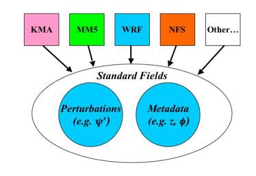
Fig. 1: Sketch of gen_be's stage0 program. Model-specific (e.g. gen_be_stage0_wrf for WRF) processing of full field forecast fields is performed to convert to perturbation fields of "standard" variables and relevant metadata, e.g. latitude, height, land/sea, etc.

Input: Model-specific forecast files.

Processing: Read forecasts, calculate x’ perturbations, transform to standard perturbation fields.

Output: File containing standard fields in specific binary format, with filename e.g. diff.2003-01-01_12:00:00 (perturbation valid at 12Z on 1 January 2003).

The standard gridpoint fields are:

Perturbations: Streamfunction y’(i,j,k), velocity potential c’(i,j,k), temperature T’(i,j,k), relative humidity r’(i,j,k), surface pressure p_s‘(i,j).

Full-fields: height z(i,j,k), latitude f(i,j) (these are required for the production of background error statistics stored in terms of physics variables, rather than tied to a specific grid. This flexibility is included in gen_be through a namelist option to define the bins over which data is averaged in a variety of ways (e.g. latitude height, gridpoints). Land-sea and orographic effects may also be represented in this way.

The calculation of streamfunction and velocity potential from input u and v fields is performed via a Fast Fourier Transform (FFT) decomposition of computed vorticity and divergence fields. Each model has it's own stage0 (only that for WRF - gen_be_stage0_wrf is supported at present) which outputs a common format so that the remaining stages below are the same for all model data.

b. gen_be_stage1 (remove mean)

This stage simply reads the difference fields output by stage0 and removes the time/bin mean from each standard field and level. The zero-mean fields are output to separate directories/files for each variable, date and member (e.g. psi/2003010112.psi.NMC contains the 3D psi field from NMC-method data, with mean removed).

Input: Perturbation fields (output of stage 0)

Processing: Remove mean for each variable/level.

Output: Standard fields: f(i,j), z(i,j,k), y’(i,j,k), c’(i,j,k), T’(i,j,k), p_s‘(i,j).

c. gen_be_stage2 (multivariate regression coefficients)

The standard control variables (i.e. those variable for which we assume cross-correlations are zero) in WRF-Var are streamfunction, "pseudo" relative humidity, and the unbalanced components of velocity potential, temperature, and surface pressure.

The “unbalanced” control variables are defined as the difference between full and “balanced” (or correlated) components of the field. In this stage of the calculation of background errors, the balanced component of particular fields is modeled via a regression analysis of the field using specified predictor fields (e.g. streamfunction). (see Wu et al 2002 for further details) The resulting regression coefficients are output for use in WRF-Var’s U_p transform, and are also used in gen_be_stage2a (see below). Currently, three regression analyses are performed resulting in three sets of regression coefficients (note: drop the perturbation notation from now on for clarity):

Velocity potential/streamfunction regression: .

Temperature/streamfunction regression: .

Surface pressure/streamfunction regression: .

Data is read from all files and sorted into bins defined via the namelist option bin_type. Regression coefficients G(k1,k2) and W(k) are computed individually for each bin (bin_type=1 is used here, representing latitudinal dependence) in order to allow representation of differences between e.g. polar, mid-latitude, and tropical dynamical and physical processes. In addition, the scalar coefficient c used to estimate velocity potential errors from those of streamfunction is calculated as a function of height to represent e.g. the impact of boundary-layer physics. Latitudinal /height smoothing of the resulting coefficients may be optionally performed to avoid artificial discontinuities at the edges of latitude/height boxes.

In summary, gen_be_stage2 proceeds as follows:

Input: Standard fields (output of stage 1).

Processing: Regression analysis to determine multivariate correlations between perturbation fields.

Output: Regression coefficients c, W, G.

d. gen_be_stage2a (unbalanced control variables)

Having computed regression coefficients, the unbalanced components of the fields are calculated as , , and . These fields are output for the subsequent calculation of the spatial covariances as described below.

Input: Standard fields (output of stage 1) and regression coefficients (output of stage 2).

Processing: Compute “unbalanced” components of selected fields.

Output: Unbalanced fields , , and .

e. gen_be_stage3 (vertical eigenvectors/eigenvalues)

The gen_be_stage3 program calculates the statistics required for the vertical component of the control variable transform of WRF-Var. This involves the projection of 3D fields on model-levels onto empirical orthogonal functions (EOFs) of the vertical component of background error covariances (Barker et al 2003).

The gen_be_stage3 code calculates both domain-averaged and local values of the vertical component of the background error covariance matrix. The definition of local again depends on the value of the namelist variable bin_type chosen. For example, for bin_type=1, a kz x kz (kz is the number of vertical levels) vertical component of B is produced at every latitude (data is averaged over time and longitude) for each control variable. Eigendecomposition of the resulting climatological vertical error covariances results in both domain-averaged and local eigenvectors E and eigenvalues . Both sets of statistics are included in the dataset supplied to WRF-Var, allowing the choice between homogeneous (domain-averaged) or local (inhomogeneous) background error variances and vertical correlations to be chosen at 3D-Var run-time (Barker et al 2003).

Having calculated and stored eigenvectors and eigenvalues, the final part of gen_be_stage3 is to project the entire sequence of 3D control variable fields into EOF space ready for calculation of power spectra.

Input: 3D (i,j,k) control variable fields: , , , and r’ (output from stage 1 and 2a).

Processing: For each variable: compute vertical component of B, perform eigenvector decomposition, and compute projections of fields onto eigenvectors.

Output: Eigenvectors E, eigenvalues L, and projected 3D (i,j,m) control variable fields: , , , and r’ for further processing of power spectra (next stage).

f. gen_be_stage4 (horizontal error correlations)

The last aspect of the climatological component of background error covariance data required for WRF-Var are the horizontal error correlations, the representation of which forms the largest difference between running WRF-Var in regional and global mode (it is however, still a fairly local change).

In global applications (gen_be_stage4_global). a spectral decomposition of the grid-point data is perfomed, and power spectra computed for each variable and vertical mode. Details of the spectral technique used to project gridpoint fields to spectral modes are given in Appendix B together with a description of the power spectra computed from the spectral modes.

In regional applications (gen_be_stage4_regional), a recursive filter is used to provide the horizontal correlations (Barker et al 2003). The error covariance inputs to the recursive filter is a correlation lengthscale (provided by gen_be_stage4_regional), and a WRF-Var namelist parameters to define the correlations shape (the number of passes through the recursive filter). The calculation of horizontal lengthscales in gen_be_stage4_regional is described in section 8c of Barker et al (2003). Note: This is the most expensive part of the entire gen_be process. Ways to reduce the computational cost are described in Appendix A (User Guide).

Input: Projected 3D (i,j,m) control variable fields: , , , and r’, and (i,j).

Processing (regional): Perform linear regression of horizontal correlations to calculate recursive filter lengthscales (see Barker et al 2003).

Processing (global): Perform horizontal spectral decomposition, and compute power spectra for each field/mode (see Appendix B).

Output (regional): Recursive filter lengthscales for each control variable, vertical mode.

Output (global): Power spectra for each control variable, vertical mode.

4. Example gen_be results

To come.

5. Tuning of Forecast and Observation Error Covariances

To come.

a. Tuning based on observation minus forecast differences

b. Variational tuning algorithms.

6. Summary and Future Work

7. References

Appendix A: gen_be User Guide

The gen_be utility is part of the WRF-Var system, and is therefore distributed as part of the WRF-Var release. The fortran codes for gen_be can be found in wrfvar/gen_be. The scripts to run these codes are in wrfvar/run/gen_be.

a. Input data

The input data for gen_be are WRF forecasts, that are used to generate model perturbations, used as a proxy for estimates of forecast error. As discussed above, for the NMC-method, the model perturbations are differences between forecasts (e.g. T+24 minus T+12 is typical for regional applications, T+48 minus T+24 for global) valid at the same time. Given input from an ensemble prediction system (EPS), the inputs are the ensemble forecasts, and the model perturbations created are the transformed ensemble perturbations.

It is important to include forecast differences from at least 00Z and 12Z through the period, to remove the diurnal cycle (i.e. do not run gen_be using just 00Z or 12Z model perturbations alone).

The inputs to gen_be are NETCDF WRF forecast output ("wrfout") files at specified forecast ranges. To avoid unnecessary large single data files, it is assumed that all forecast ranges are output to separate files. For example, if we wish to calculate BE statistics using the NMC-method with T+24-T+12 forecast differences (default for regional) then by setting the WRF namelist.input options history_interval = 12, and frames_per_outfile =1 we get the necessary output datasets. If the files are then arranged as follows, the gen_be.csh script can be used without significant modification to calculate the necessary "perturbations".

Example directory/files structure for a sub-period of our Katrina 12km domain (450 x 350 x 51 gridpoints):

-rw-r--r-- 1 dmbarker users 394105664 Nov 6 07:24 2005082700/wrfout_d01_2005-08-28_00:00:00

-rw-r--r-- 1 dmbarker users 394105664 Nov 6 11:00 2005082712/wrfout_d01_2005-08-28_00:00:00

-rw-r--r-- 1 dmbarker users 394105664 Nov 6 15:01 2005082712/wrfout_d01_2005-08-28_12:00:00

-rw-r--r-- 1 dmbarker users 394105664 Nov 6 18:15 2005082800/wrfout_d01_2005-08-28_12:00:00

-rw-r--r-- 1 dmbarker users 394105664 Nov 6 21:14 2005082800/wrfout_d01_2005-08-29_00:00:00

-rw-r--r-- 1 dmbarker users 394105664 Nov 9 22:17 2005082812/wrfout_d01_2005-08-29_00:00:00

-rw-r--r-- 1 dmbarker users 394105664 Nov 10 02:15 2005082812/wrfout_d01_2005-08-29_12:00:00

-rw-r--r-- 1 dmbarker users 394105664 Nov 10 07:12 2005082900/wrfout_d01_2005-08-29_12:00:00

-rw-r--r-- 1 dmbarker users 394105664 Nov 10 10:43 2005082900/wrfout_d01_2005-08-30_00:00:00

-rw-r--r-- 1 dmbarker users 394105664 Nov 10 16:29 2005082912/wrfout_d01_2005-08-30_00:00:00

-rw-r--r-- 1 dmbarker users 394105664 Nov 10 19:29 2005082912/wrfout_d01_2005-08-30_12:00:00

-rw-r--r-- 1 dmbarker users 394105664 Nov 11 01:43 2005083000/wrfout_d01_2005-08-30_12:00:00

-rw-r--r-- 1 dmbarker users 394105664 Nov 11 04:43 2005083000/wrfout_d01_2005-08-31_00:00:00

-rw-r--r-- 1 dmbarker users 394105664 Nov 21 00:19 2005083012/wrfout_d01_2005-08-31_00:00:00

-rw-r--r-- 1 dmbarker users 394105664 Nov 21 03:29 2005083012/wrfout_d01_2005-08-31_12:00:00

-rw-r--r-- 1 dmbarker users 394105664 Nov 21 08:23 2005083100/wrfout_d01_2005-08-31_12:00:00

-rw-r--r-- 1 dmbarker users 394105664 Nov 21 12:40 2005083100/wrfout_d01_2005-09-01_00:00:00

-rw-r--r-- 1 dmbarker users 394105664 Nov 21 17:37 2005083112/wrfout_d01_2005-09-01_00:00:00

-rw-r--r-- 1 dmbarker users 394105664 Nov 21 20:36 2005083112/wrfout_d01_2005-09-01_12:00:00

-rw-r--r-- 1 dmbarker users 394105664 Nov 22 02:45 2005090100/wrfout_d01_2005-09-01_12:00:00

....

-rw-r--r-- 1 dmbarker users 394105664 Nov 21 20:36 2005092700/wrfout_d01_2005-09-28_00:00:00

-rw-r--r-- 1 dmbarker users 394105664 Nov 22 02:45 2005092712/wrfout_d01_2005-09-28_00:00:00

In the above example, a whole month (00Z 28 Aug to 00Z 28 Sep. 2005) of forecasts, every 12 hours are supplied to gen_be to estimate forecast error covariances. The minimum number of forecasts required depends on the application, number of gridpoints, etc. Month-long (or longer) datasets are typical for the NMC-method.

a. Compilation

As with WRF and WRF-Var, there are two steps to compiling gen_be. From within the wrfvar directory, one types

./configure be

At the prompt, choose the single processor option (gen_be is a serial code, at least at the code level). This will produce a configure.wrf file containing the necessary compile options for your machine. Secondly, type

./compile be

This will compile all the gen_be codes. Compilation should not take more than 30s.

b. gen_be scripts

The gen_be utility is run through the interface script gen_be.csh, which calls a number of other scripts for various stages. As with WRF_Var, there are a large number of job parameters (e.g. code/data directories, namelist options) that can be set via environment variables. Each stage may also be switched off/on by [un]commenting the appropriate variable, e.g. setenv RUN_GEN_BE_STAGE0.

Note 1: Further details of particular namelist parameters may be found in the self-documented scripts.

Note 2: The output from gen_be_stage0_wrf.csh will a series of unformatted perturbation files containing the "standard fields" (psi, chi, T, rh, ps), e.g the file "diff.2005-09-02_00:00:00" contains T+24-T+12 fcst differences valid at 2005090200, transformed to standard fields.

Note 3: For global applications, gen_be runs relatively quickly (typically a few hours on 1PE for e.g. T213 data). For regional applications, the cost is typically higher - predominantly due to the calculation of correlation lengthscale (gen_be_stage4_regional). There are two ways to decrease the run-time of gen_be_stage4_regional:

i. Run separate gen_be_stage4_regional jobs on seperate processors, i.e. parallelize at the script level. This is possible because the calculation of lengthscales for each variable/vertical mode is independent, so one could in principle run num_variables * num_vertical_modes independent gen_be_stage4_regional jobs (e.g. ~200 parallel jobs for the Katrina case above). The gen_be.csh script includes two environment variables (NUM_JOBS and MACHINES) to do this. Setting NUM_JOBS to be greater than 1 will cause the script to spawn jobs on nodes defined in the MACHINES list. Note - this has only been tested to date on linux platforms.

ii. Reduce the number of calculations within gen_be_stage4_regional. The expense of this stage is large due to the point-to-point calculation of correlations between gridpoints. This is already optimized in the sense that only one diagonal of the grid are used in the calculation of the correlation (<x_i x_j>=<x_j x_j >). The cost may be further reduces via the namelist parameter STRIDE, which skips every stride points on the grid, i.e. "do i/j = 1, dim1/2, stride". Of course, this will change the scientific results, but for large domains with sufficient input data (e.g. month long series), the differences between strides of 1 (default) and 2, 4 may be scientifically insignificant with huge reduction (4x, 16x) in CPU requirements. Experience with a particular domain is required to define the optimal stride value.

Appendix B: The Spectral Technique

a. Introduction

The use of spectral transformations in variational data assimilation relies on the basic assumption that error correlations of the chosen "control variables" are homogeneous and isotropic. Indeed, the choice of control variables is partly based on the degree of homogeneity and isotropy of particular variables. For example, streamfunction and velocity potential satisfy these conditions more than the u-, and v- components of the wind field at least in the extra-tropics (see Ingleby 2001 and references).

It is important to note that the use of a spectral transform does not imply error covariances are also homogeneous (which they are not in reality) as one can still impose synoptically-, or geographically-dependent error variances. In addition, there are numerous ways to impose anisotropic error correlations (e.g. grid-transformations, additional control variables, wavelets, 4D-Var) while still retaining the benefits (data compression, scalability) of the spectral method. For these reasons, the spectral method is used to model horizontal error correlations in global applications of WRF-Var.

b. Theory of the Spectral Transform

Any real, continuous function on a sphere can be represented by the summation

(A1)

where the are the complex, spectral coefficients of , longitude , and latitude . The two indices m and n are the zonal (Fourier) and total (Legendre) wavenumbers respectively. The spherical harmonic functions are given by

(A2)

where , and the are the associated Legendre polynomials, described in further detail in the next subsection. In practice, the summations in (A1) must be truncated at finite limits , and . In triangular truncation, the limits are equal i.e. . Alternative truncations may be applied in order to introduce a degree of anisotropy (Jarraud and Simmons 1991).

The inverse of (A1) (i e. the transform from gridpoint to spectral space) is best illustrated in two stages. Firstly, a Fourier transformation of the real field into a complex, intermediate state is performed via (fast) Fourier transformation

, (A3)

Secondly, a Legendre transformation is performed to transform the complex fields into spectral modes

(A4)

The calculation of spectral coefficiencts is exact if the input gridpoint field is on Gaussian latitudes (in which case the interpolation weights Wj are the Gaussian weights). In contrast, if the gridpoint field is on regular latitudes, then there is an error in the gridpoint to spectral conversion performed by (A4) (and the interpolation weights Wj are the cosine of the latitude multiplied by the latitudinal grid spacing (in radians). The differences between Gaussian and regular latitudes are confined mainly to a few points near the pole.

Note: There is no error in the spectral to grid transformation (A1) performed within 3D-Var, and so there is no need to perform 3D-Var on Gaussian latitudes (the final spectral analysis increments can be projected back to whatever grid is chosen to run the forecast with no error). The error introduced in (A4) does however affect the calculation of background error statistics. To remove this error completely, all that is required is to produce the forecast differences that are used to create background error statistics on Gaussian latitudes.

c. Power Spectra

If the covariances of are homogeneous and isotropic, then the spectral coefficients are uncorrelated, and their variance is independent on m (Boer 1983). In the case, the power spectrum

(A5)

gives the total variance at total wavenumber n. The second equality in (A5) follows assuming the function is real. The total variance V over all wavenumbers is then given by . In WRF 3/4D-Var, we wish to reduce the condition number of the minimization problem. In the spectral transform, this can be achieved by dividing the spectral coefficients by their expected modal standard deviation, i.e. the normalized, spectral control variables of a real function are given by

. (A6)

d. Associated Legendre Polynomials

The values of are calculated via recursion relationships. In WRF 3/4D-Var, two methods are employed, based on earlier studies using the Met. Office's 3D-Var system. Firstly, for the relation

(A7)

is used. The coefficients used in (A7) are given by

, (A8a)

,(A8b)

(A8c)

for (Jarraud and Simmons 1991). Eqn. (A7) is mathematically stable. However, it requires and to calculate and hence cannot be used for m = 0, 1. For these values, the following alternative recursion relation is used (Press et al, 1986):

(A9a)

(A9b)

. (A9c)

Eqns. (A9) are not used for higher m as initial single-precision experiments indicate numerical instability for .

Numerous properties and symmetries of associated Legendre polynomials exist, and can be used to reduce the number of values that need to be calculated, and stored. The following are currently used in WRF 3/4D-Var:

, if , (A10)

The storage savings can be illustrated for typical values J=100 latitude points and m=n=99. Without using (A10), there are values of . Using the properties of (A10), the number of required stored values is i.e. a factor of ~8 less.