Running 4D-VAR

Reference: Download the tutorial presentation

Source code

Get the pre-compiled code, if you have not done so.

WRFDA/var/build/da_wrfvar.exe

is the executable that will be used in the 4D-VAR session. The pre-compiled code was compiled for 4DVAR, so if you are using code you compiled yourself, make sure this executable was compiled for 4DVAR. Otherwise, 4DVAR assimilation will not work!

Choice of your working directory

We recommend running each session in a separate directory, so that it will be easier to check for the necessary input files and look for what output files are created after a successful run.

We recommend you create /home/ec2-user/workdir/4dvar and cd there to be your working directory for this session.

mkdir /home/ec2-user/workdir/4dvar
cd /home/ec2-user/workdir/4dvar

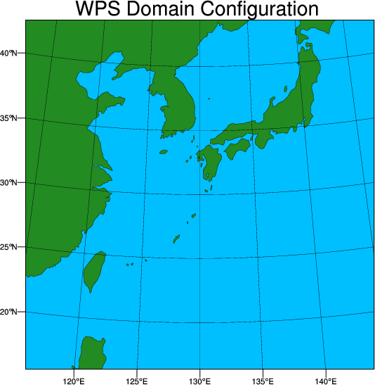
For running 3D-VAR, the 3 major input files are observations (ob.ascii), background error statistics (be.dat) and first guess (fg). For 4D-VAR, the similar concept holds except that now the observations need to be processed into multiple time-slot files. This case utilizes a western Pacific, 51x51 gridpoints, 31 vertical levels, and 60km resolution (it can be found at /home/ec2-user/test_data/4dvar). This is a much lower resolution than should normally be run to see good results; the test is kept small for tutorial purposes. The exact area of the domain is shown at right. It features Tropical Storm Nanmadol striking southern Japan on July 04, 2017. Due to the low resolution, the typhoon is not well-resolved in this case, but you should be able to see it in the wind field with the ncview utility.

• Observations

  You should already have created observation files for this case in the obsproc practice; if you haven't, go back and finish the exercise.

• First guess

  /home/ec2-user/test_data/4dvar/rc/2017070400/wrfinput_d01
  /home/ec2-user/test_data/4dvar/rc/2017070400/wrfbdy_d01

• Background error statistics

  For this exercise, we will use the built-in CV3 option (included in the source code under /home/ec2-user/compiled_code/WRFDA-v4.1.2/var/run/be.dat.cv3)

Compared to 3DVAR, several more input files are necessary for 4DVAR runs. Most of these are static data files, necessary for running the nonlinear model as part of the 4DVAR assimilation.

ln -sf /home/ec2-user/compiled_code/WRFDA-v4.1.2/run/RRTM_DATA_DBL ./RRTM_DATA

ln -sf /home/ec2-user/compiled_code/WRFDA-v4.1.2/run/*.TBL .

Link first guess and boundary files. The "wrfinput_d01" file should be linked both as "fg" and "wrfinput_d01". wrfbdy_d01 (WRF boundary conditions file) is also needed for running the nonlinear model.

ln -sf /home/ec2-user/test_data/4dvar/rc/2017070400/wrfinput_d01 ./fg

ln -sf /home/ec2-user/test_data/4dvar/rc/2017070400/wrfinput_d01 .

ln -sf /home/ec2-user/test_data/4dvar/rc/2017070400/wrfbdy_d01 .

Link observation files (if you haven't created these yet, go back and finish the OBSPROC exercise)

ln -sf /home/ec2-user/workdir/obsproc_4dvar/obs_gts_2017-07-04_00:00:00.4DVAR ./ob01.ascii

ln -sf /home/ec2-user/workdir/obsproc_4dvar/obs_gts_2017-07-04_01:00:00.4DVAR ./ob02.ascii

ln -sf /home/ec2-user/workdir/obsproc_4dvar/obs_gts_2017-07-04_02:00:00.4DVAR ./ob03.ascii

ln -sf /home/ec2-user/workdir/obsproc_4dvar/obs_gts_2017-07-04_03:00:00.4DVAR ./ob04.ascii

Link the background error file (we will use the built-in CV3 option here for demonstration purposes)

ln -sf /home/ec2-user/compiled_code/WRFDA-v4.1.2/var/run/be.dat.cv3 ./be.dat

A very basic namelist.input for running the 4D-VAR tutorial case is available at /home/ec2-user/test_data/4dvar/namelist.input

cp /home/ec2-user/test_data/4dvar/namelist.input .

vi namelist.input

Pay special attention to the following namelist variables.

&wrfvar1
var4d=true,
var4d_lbc=false,
var4d_bin=3600,
/
&wrfvar18
analysis_date='2017-07-04_00:00:00",
/
&wrfvar21
time_window_min="2017-07-04_00:00:00",
/
&wrfvar22
time_window_max="2017-07-04_03:00:00",
/
&time_control
force_use_old_data=true,
run_hours=3,
start_year=2017,
start_month=07,
start_day=04,
start_hour=00,
end_year=2017,
end_month=07,
end_day=04,
end_hour=03,
interval_seconds=10800,
/
&domains
time_step=360,
e_we=51,
e_sn=51,
e_vert=31,
dx=60000,
dy=60000,
/
&dynamics
hybrid_opt=0,
use_theta_m=0,
etac=0.0,
/
&perturbation
trajectory_io=true,
enable_identity=false,
jcdfi_use=true,
jcdfi_diag=1,
jcdfi_penalty=1000.0,
/

mpirun -np 8 /home/ec2-user/compiled_code/WRFDA-v4.1.2/var/build/da_wrfvar.exe >& var4d.log &

The "&" at the end of the above command tells WRFDA to run in the background. Because the command line is now usable even as WRFDA runs, you can use the "tail" command to follow the progress of WRFDA as it writes the log files:

tail -f rsl.out.0000

This exercise will take about 4 minutes to complete on the AWS computers. Press control+c at any time to quit "tail"

When WRFDA is completed, you should see the same diagnostic files as you saw for 3dvar. Check the rsl.out.0000 file if you haven't already. You will notice a lot more messages from the tangent linear and adjoint models that can clutter up the file. If you just want to see the minimization statistics, try the command

grep minimize_cg rsl.out.0000

The output of this command will be just the minimization statistics with the columns from left-to-right representing the outer loop number,the inner loop iteration number, the cost function for that step, the gradient for that step, and the difference from the previous step:

minimize_cg   1   0   7.263276050404636D+03   1.250191294554293D+03   0.000000000000000D+00
minimize_cg   1   1   6.682097218012141D+03   4.641977504963150D+02   7.436812685625593D-04
minimize_cg   1   2   6.472266141658221D+03   3.361329765527207D+02   1.947572981557830D-03
minimize_cg   1   3   6.315595518791810D+03   3.057245254282243D+02   2.773290238826363D-03
minimize_cg   1   4   6.129124104747037D+03   3.320964829535927D+02   3.990080896054300D-03
minimize_cg   1   5   5.990263364617907D+03   2.402058753754224D+02   2.518146071560523D-03
minimize_cg   1   6   5.883601642102399D+03   1.772414412585168D+02   3.697186314395040D-03
minimize_cg   1   7   5.799206385677896D+03   1.811033252579398D+02   5.373007996992452D-03
minimize_cg   1   8   5.709416960237148D+03   1.746947602013142D+02   5.475229643260147D-03

WRFDA 4DVAR has the option to add an additional cost function term based on the lateral boundary conditions. You can activate it by setting var4d_lbc=true in &wrfvar1, and linking the following files.

ln -sf /home/ec2-user/test_data/4dvar/rc/2017070403/wrfinput_d01 ./fg02

cp ./fg02 ./ana02

"fg02" and "ana02" are the same file, and are the "first guess" field for the same domain at the end of the 4DVAR assimilation window (in this case, the analysis at 2017-07-04 03Z). Run the case again and see if you notice any differences in the output (especially the cost_fn and grad_fn files).

You are now done with the basic 4DVAR practice case. If you still have time, you can try some additional exercises below:

Additional practice

Try using PREPBUFR data instead of ASCII format data. Since PREPBUFR files from GDAS contain 6 hours of data which is different from our 6-hour assimlation window (PREPBUFR files contain data from 21z–03z, 03z–09z, etc.) you will need to link two different observation files to cover the whole assimilation window:

ln -sf /home/ec2-user/test_data/4dvar/ob/2017070400/gdas1.t00z.prepbufr.nr ./ob01.bufr

ln -sf /home/ec2-user/test_data/4dvar/ob/2017070406/gdas1.t06z.prepbufr.nr ./ob02.bufr

Radiance assimilation works in much the same way, since radiance data in GDAS BUFR files follows the same time window conventions.

ln -sf /home/ec2-user/test_data/4dvar/ob/2017070400/gdas1.t00z.1bamua.tm00.bufr_d ./amsua01.bufr

ln -sf /home/ec2-user/test_data/4dvar/ob/2017070406/gdas1.t06z.1bamua.tm00.bufr_d ./amsua02.bufr

Note that the AMSU-A radiances from NOAA-18, NOAA-19, METOP-A, and METOP-B can be used for this domain. The following namelist options are critical in order to choose the correct instruments:

&wrfvar14
rtminit_nsensor = 4,
rtminit_platform = 1, 1, 10, 10,
rtminit_satid = 18, 19, 1, 2,
rtminit_sensor = 3, 3, 3, 3,
thinning_mesh = 120.0, 120.0, 120.0, 120.0,
/

Don't forget to change additional namelist options (ob_format=1) and link the necessary radiance files/directories! Reference the 3DVAR and radiance practice if you forgot how, or you can check the Users Guide.

After running the test, try to determine how many observations were used and how many were rejected from each AMSU-A instrument using the following commands:

grep -A 2 'ngood(:)\|nrej(:)' 01_qcstat_metop-2-amsua_*
grep -A 2 'ngood(:)\|nrej(:)' 01_qcstat_metop-1-amsua_*
grep -A 2 'ngood(:)\|nrej(:)' 01_qcstat_noaa-18-amsua_*
grep -A 2 'ngood(:)\|nrej(:)' 01_qcstat_noaa-19-amsua_*

Each 01_qcstat_* file is for one satellite platform and for one of the four observation bin windows. We can see that this regional domain is sparsely covered by polar orbiting platforms in this short three hour assimilation window.

---

Try setting up a different 4D-VAR run using CONUS60 case (/home/ec2-user/test_data/CONUS60) and compare the results with the 3D-VAR run. Use the same namelist from the 3dvar case, and modify the following settings:

cp /home/ec2-user/test_data/CONUS60/namelist.input.3dvar ./namelist.input

vi namelist.input

Pay special attention to the following namelist variables, which are essential for 4DVAR runs

&wrfvar1
var4d=true,
var4d_lbc=false,
var4d_bin=3600,
/
&wrfvar6
ntmax=5 # for testing purpose only; this reduces the maximum iterations, since this 4DVAR case takes a long time to run
/
&wrfvar18
analysis_date="2008-02-05_12:00:00",
/
&wrfvar21
time_window_min="2008-02-05_12:00:00",
/
&wrfvar22
time_window_max="2008-02-05_18:00:00",
/
&time_control
force_use_old_data=true,
run_hours=6,
start_year=2008,
start_month=02,
start_day=05,
start_hour=12,
end_year=2008,
end_month=02,
end_day=05,
end_hour=18,
interval_seconds=21600,
/
&domains
time_step=360,
e_we=90,
e_sn=60,
e_vert=41,
dx=60000,
dy=60000,
/
&dynamics
diff_opt=1,
km_opt=4,
hybrid_opt=0,
use_theta_m=0,
etac=0.0,
/
&perturbation
trajectory_io=true,
enable_identity=false,
jcdfi_use=true,
jcdfi_diag=1,
jcdfi_penalty=1000.0,
/
&bdy_control
specified=true,
real_data_init_type=3,
/

• Observations

  ln -sf /home/ec2-user/test_data/CONUS60/ob/200802051*/ob0*.ascii .
  

• First guess

  ln -sf /home/ec2-user/test_data/CONUS60/rc/2008020512/wrfinput_d01
  ln -sf /home/ec2-user/test_data/CONUS60/rc/2008020512/wrfbdy_d01

  ln -sf /home/ec2-user/test_data/CONUS60/rc/2008020512/wrfinput_d01 ./fg

• Background error statistics

  ln -sf /home/ec2-user/test_data/CONUS60/be/be.dat

You can also try assimilating PREPBUFR and radiance data, as described above. Those observation files can be found in the appropriate sub-directories in /home/ec2-user/test_data/CONUS60/ob