NCAR TN 448+STR

This NCAR Technical Note supplements the paper "Inferences of Predictability Associated with Warm Season Precipitation Episodes" by Carbone et al. (2001). It includes a superset of the meridionally-averaged and zonally-averaged rainfall rate diagrams that underlie the Carbone et al. study and explains the construction of these Hovmöller diagrams. Additional monthly and seasonal statistics related to the precipitation structures found within the Hovmöller diagrams are computed. The analysis period spans the warm season months of May through August, 1996 through 2000.

Acknowledgements

This research was sponsored by National Science Foundation support to the U.S. Weather Research Program. The authors are deeply appreciative for assistance received from the National Climatic Data Center, the website of NOAA/CIRES Climate Diagnostics Center at U. of Colorado, S. Goodman of NASA's Marshall Spaceflight Center, NOAA/CIRA at Colorado State University, NOAA/NESDIS, and our sister organizations at NCAR/UCAR, namely the Research Applications Program and COMET. These organizations provided critical access to datasets, without which this study would have been impossible. Comments from L. J. Miller of MMM/NCAR have also greatly improved this Technical Note.

1. Introduction

One of the biggest problems facing atmospheric scientists today is the accurate representation and prediction of summertime precipitation. While faster computers and better analytical models have led to significant improvement in wintertime forecasts, our inadequate representation of dynamical and microphysical processes important to summertime convection has meant slower progress in the arena of warm season quantitative precipitation forecasts.

This Technical Note supplements the Carbone et al. (2001) study, for which meridionally-averaged composites of national radar reflectivity were used to compile seasonal statistics on the zonal span, phase speed, duration and recurrence frequency of temporally and spatially coherent rainfall episodes. At the upper end of this episode spectrum are precipitation events that persist longer than 24 h or have zonal span exceeding 1250 km. Carbone et al. found that these long-lived events are not exceedingly rare; their recurrence interval is only two days. Their characteristic phase speed cannot be explained either by transient synoptic disturbances or steering winds, and their duration exceeds the lifespan of a single mesoscale convective complex (e.g. Laing and Fritsch 1997). Inspection of radar loops usually reveals a chain of mesoscale convective systems (MCSs) responsible for the longer episodes (>36 h), but further research is necessary to fully explain their longevity. Twelve- to 36-h forecasts of summertime precipitation stand to benefit from a better physical understanding of the linkage between these successive MCSs. Interested readers should refer to Carbone et al. (2001) for further motivation and background material.

The remainder of the document consists of three text sections, a table section, plus four Appendices. The following section describes the principal data set used in the Carbone et al. (2001) study. The next section details the process of constructing longitude-time and latitude-time sections from the radar reflectivity data. The steps taken to analyze the longitude-time sections (Hovmöller diagrams) are found in the final section. The Appendices contain Hovmöller diagrams produced for the years 1996 through 2000 as well as related analyses for seasonal, monthly, and daily periods.

2. NOWrad™ MASTER15 Product

This study relies heavily on a national radar reflectivity composite produced by Weather Services International Corporation (WSI). Known as the NOWrad™ MASTER15, this product is synthesized every 15 minutes from all operational National Weather Service (NWS) radars (the WSR-88D network). The data undergoes three levels of quality control at WSI: two at the single-site level and one at the national composite level. The first two levels are completed via computer algorithms, while the third and final stage involves a radar technician who attempts to manually remove anomalous propagation echoes, ground clutter, and other miscellaneous errors. WSI also produces a product every five minutes with no manual corrections. However, the positive impact of the third level of quality control is too great to justify using the 5-minute product exclusively in our study. The 5-minute resolution product was used primarily to fill data gaps in our 15-minute resolution NOWrad™ product archive. These data gaps accounted for only 0.4% of the total time reported here.

Using all available tilt angles, WSI merges WSR-88D radar reflectivity volumes into a two-dimensional mosaic over the U.S. with sixteen 5-dBZ_e reflectivity levels, beginning with level 0 (0-5 dBZ_e). Although the exact algorithm by which WSI integrates single-site radar data into a national composite is proprietary information, it is generally understood that the mosaic contains the highest reflectivity found within the vertical column centered on each grid point. The reflectivity data is mapped to a cylindrical equidistant projection with 1837 rows and 3661 columns, and a grid spacing of approximately 2 km. See Table 1 for additional NOWrad™ MASTER15 specifications.

Our NOWrad™ MASTER15 national radar composite archive was obtained from the Global Hydrology Resource Center (GHRC) at the Global Hydrology and Climate Center, Huntsville, Alabama. The GHRC maintains a 5-year archive of NOWrad™ MASTER15 products dating back to 10 October 1995. At the time of this writing, data may be accessed through the website: http://ghrc.msfc.nasa.gov/hydro.html or by mail:

GHRC User Services Office
Global Hydrology and Climate Center
320 Sparkman Dr
Huntsville, AL 35805

In order to conserve disk space, GHRC reformatted and stored the NOWrad™ data in Hierarchical Data Format (HDF) format as run length encoded raster 8 images. Information on decoding the HDF data structure is available on the GHRC web site, and the HDF software library is at http://hdf.ncsa.uiuc.edu.

As stipulated by the contractual agreement between the GHRC and WSI, use of this data set is restricted to educational (including K-12) or research, non-commercial purposes. Researchers are prohibited from redistributing it. Therefore, interested parties must contact the GHRC to access the national radar composites used in this study.

3. Construction of Hovmöller Diagrams

The NOWrad™ gridded radar data were used to create Hovmöller diagrams of estimated rainfall rate over the contiguous U.S. for the warm seasons of 1996 to 2000. In general, a Hovmöller diagram maps a scalar quantity to distance-time space. The scalar variable is averaged along the spatial dimension (or dimensions) orthogonal to the spatial dimension plotted in the Hovmöller diagram. Among other uses, these diagrams have been used in the past to diagnose patterns and isolate signals in equatorial convection (e.g. Lau and Peng 1987; Hayashi and Nakazawa 1989).

Figure 1. This flowchart illustrates the method used to compute longitude-time sections of radar-estimated rainfall rate (i.e. the zonal Hovmöller diagrams.) See text for details.

In our case, we begin with a time series of radar reflectivity mapped to a latitude/longitude grid (the NOWrad™ MASTER15 product). The two spatial dimensions are reduced to one dimension using a procedure illustrated in Fig. 1. First, the region of interest is divided into narrow strip-like subdivisions. After converting to rainfall rate, the arithmetic average is taken of the rainfall rate values within each strip. This average rainfall rate, in turn, becomes one data point in the final Hovmöller diagram. In Fig. 1, the distance dimension of the Hovmöller diagram happens to be longitude, making this a zonal Hovmöller diagram. In the zonal Hovmöller diagrams, meridional information is lost in the averaging process, effectively eliminating this spatial dimension. Conversely, in the meridional Hovmöller diagrams, zonal information is lost. Throughout this document, distance-time section and Hovmöller diagram are used interchangeably. The terms longitude-time section and zonal Hovmöller diagram are also synonymous.

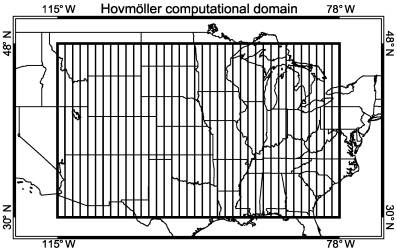
Our region of interest (delineated by the solid, bold rectangle in Fig. 2) lies between 30 and 48 N latitude and between 115 and 78 W longitude. The vertical lines drawn across the domain in Fig. 2 illustrate the orientation of the subdivisions for zonal Hovmöller diagrams. For clarity, subdivisions are shown with 1°-wide vertical strips whereas, in actuality, there are 740 strips of width 0.05-degrees between 115 and 78 W. Due to the convergence of meridians, the zonal width varies from 4.8 km at 30 N to 3.7 km at 48 N. For the meridional Hovmöller diagrams, the domain of interest is divided into subdivisions that stretch from 115 to 78 W and are 0.05° (5.6 km) in north-south extent. Three-hundred-sixty meridional subdivisions lay between 30 and 48 N.

In order to transform radar reflectivity factor in dBZ_e to estimated rain rate R in mm h^-1, the logarithmic reflectivity was linearized to Z_e (mm⁶m^-3) and then converted to R using an exponential relationship:

The multiplicative coefficient, 300, seems to render a relatively small net bias in radar-estimated national rainfall when compared to rainfall analyses derived from rain gauges (Klazura et al. 1999). While using a single Z_e-R relationship is fraught with uncertainty, quantitative precipitation estimation was not central to our study. The radar data was primarily used to determine the zonal span and duration of rainfall events.

Finally, to produce the actual Hovmöller diagrams, the estimated rainfall rates were plotted in longitude-time (latitude-time) space for the zonal (meridional) Hovmöller diagrams, with each rainfall rate pixel centered between the longitude (latitude) bounds of its representative subdivision. Zonal and meridional Hovmöller diagrams for each of the warm seasons (May through August) from 1996 to 2000 are included in Appendix A.

4. Rain Streak Statistics

We perform various analyses on the Hovmöller diagram data to quantify rainfall event coherency, duration, zonal distance (hereinafter referred to as "span"), and rate of propagation.

To identify events, rectangular autocorrelation functions were fit to the rainfall rate data in Hovmöller space (illustrated in Fig. 3). The bounded functions are uniform in one dimension and cosine-weighted in the other:

Its spatial dimensions and amplitude were chosen to match that of an archetypal rainfall rate "streak" segment in Hovmöller space. The two dimensional function was centered on a given longitude/time coordinate and rotated at 1-degree intervals through all angles (except for slope zero) until the linear correlation between the function weighting and the underlying rainfall rate values was maximized. The function was stepped through all longitude/time coordinates at 0.2°/15 min intervals. Sequences of contiguous "fits" defined the coherent span, duration, and propagation characteristics for each event. The minimum rainfall rate threshold to initiate a "fit" was 0.1 mm h^-1 and the correlation coefficient had to be 0.3 or higher. The zonal span and duration of the streaks were determined by the coordinates of the first and last "fit" in the contiguous sequence. To convert from degrees longitude to kilometers, we used the relation

which is valid at the center latitude of our domain (39 N). Shown in Fig. 3 are several examples of "fits" during a two-day period in June 1998.

For the purpose of zonal span and duration statistics (as summarized in Tables 2-4), the uniformly weighted dimension of the autocorrelation function was only 15 grid points, or ~3 degrees, consistent with the size of an individual mesoscale convective system and able to exceed the correlation threshold near the beginning and end of a rainfall streak. Along the longitude axis, 15 grid points cover exactly 3°. For the purpose of propagation statistics (e.g. Table 5), the uniform dimension was extended to 60 grid points, or ~12°, in order to have a stable measure of sustained movement for significant rainfall episodes with a zonal span of order 1000 km. The span of the autocorrelation function in the cosine-weighted dimension in both applications was 12 grid points, equivalent to ~3 h rainfall duration at a given longitude. The length, width, and shape of the autocorrelation functions are somewhat arbitrary; however, adjusting these parameters does not significantly alter the rainfall event statistics.

Most major episodes in Hovmöller space continuously produce detectable precipitation throughout their lifetime. However, some events exhibit intermittency while retaining phase speed coherence. Consider an eastward propagating, dissipating squall line whose remnant cold pool/gust front initiates another MCS 100 km downstream. The two precipitation entities are causally related and should be viewed as a single long-lived precipitation episode. However, our algorithm may accidentally classify them as two separate events if the meridionally-averaged rainfall rate dips below 0.1 mm h^-1 before the second MCS forms. This type of error was fixed by studying radar loops and determining whether the two events were causally linked (perhaps by a cold pool whose weak radar return was lost in the meridional average). If the events were indeed linked, then the two rainfall streak segments in Hovmöller space were reclassified as a single episode. Subjectively determined corrections such as this, which took the form of disconnects and reconnects of precipitation entities, occurred in approximately 2% of all cases.

The coordinates of each point in the scatter plot in Fig. 4 represent the zonal span and duration of an individual rainfall streak during the period May through August, 1997 to 2000. The median zonal span/duration ratio for the population of rainfall streaks with span >1000 km and duration >20 h was 14.3 m s^-1, represented by the solid line in Fig. 4.

In Table 2, we employ recurrence frequency as the means to express rainfall streak zonal span and duration for the "longest" 10% of all rainfall episodes. Table 2 lists the rainfall streak zonal span (km) and duration (h) corresponding to several recurrence frequencies.

The cumulative probability histogram of rainfall streak zonal span, as defined earlier, is shown in Fig. 5 for the years 1997 through 2000, May through August. The histogram exhibits a continuum of events with decreasing frequency out to 2600 km, the approximate distance from the western Great Plains to the eastern edge of the domain. For the purposes of parameterization, the cumulative distribution may be approximated by a power law of the form

where N(S) is the number of rainfall streaks of zonal span > S (km), N₀ is the total number of streaks, and L = 0.001 km^-1.

Figure 5 also exhibits the cumulative probability histogram of rainfall streak duration. As with rainfall streak zonal span, the cumulative distribution for streak duration may be approximated by a power law

where D is duration (h) and G = 0.05 h^-1. Equations 4 and 5 can be combined to produce a characteristic phase speed

Table 3 lists a pair of zonal phase speeds beneath each year. Both speeds were derived by dividing a median zonal span by a median duration for that particular year. The median values for the first row were taken from all eastward moving rainfall streaks (for a particular year), while the median values for the second set of numbers were drawn from the population of rainfall streaks with zonal span > 1000 km and duration > 20 h.

Table 4 summarizes three additional sets of phase speed estimates, stratified according to recurrence frequency. The top row within each recurrence frequency is simply the span/duration ratio from the span, duration couplets in Table 2. The middle row within each recurrence frequency is the exceedance speed, defined as the span/duration ratio that is equaled or exceeded with a particular frequency. For example, during the 123-day period of record in 1997, the span/duration ratio for a rainfall streak exceeded 23.7 ms^-1 about 123 times, or once per day.

The bottom row within each recurrence frequency arose from scatter plots of rainfall streak duration and zonal span for individual years. This process is illustrated for 1997 in Fig. 6. First, the locations in the scatter plot whose coordinates share a particular recurrence frequency were established. As seen in Fig. 6, these anchor points were marked with bold dots. Next, the constant phase speed line was drawn whose slope equaled the median span/duration ratio for long rainfall events (span > 1000 km and duration > 20 h) for that year. On either side of each anchor point, a pair of lines was drawn. Both lines were perpendicular to the constant phase speed line and equidistant from their anchor point. Note that all events along one of these lines share a characteristic length, defined as a linear combination of duration and zonal span. The lightly shaded bands in Fig. 6 that straddle each anchor point do not overlap and each band encompasses up to 25 data points (depending on the density of the data points). Once the bands were established, the median span/duration ratio for each band was entered into the bottom row of phase speed estimates for each recurrence frequency in Table 4. The "one per month" category is not shown since there were almost no data points at this recurrence frequency. The median span/duration ratio within each recurrence frequency band was comparable to the phase speed derived from the span, duration couplets in Table 2 because the sample of rainfall streaks within each particular recurrence frequency band was not skewed towards fast or slow phase speeds.

For the years 1997 through 2000, we examined both zonal span and duration properties from 5406 rain streaks over 492 warm season days, or approximately 11 per day. In addition, we measured phase speeds and compared them to the phase speed of upper tropospheric anomalies and zonal "steering-level" winds. This process is described in the next section.

4.1 Zonal phase speed of large-scale forcing

Using images provided by the NOAA-CIRES Climate Diagnostics Center[1], we examined 1998 and 1999 NCEP 2.5° gridded analyses in latitude bands corresponding to the largest convective events. We compiled statistics on the zonal speed of 30 kPa anomalies and "steering" winds at 70, 50, 40, 30, and 25 kPa (Table 5).

The zonal speed of 30-kPa meridional wind anomalies served as a proxy for zonal speed of synoptic-scale forcing. We examined longitude-time sections of meridional wind anomalies at 30 kPa, such as Fig. 7. This field usually revealed a phase speed signal, though its amplitude and clarity varied. On those occasions when meridional wind anomalies at 30 kPa failed to reveal a clear phase speed signal, the examination of other upper level anomalies (geopotential height, temperature, etc.) sometimes helped define the phase speed.

The median zonal phase speed of synoptic-scale forcing was drawn from 45 estimates. Each of the 45 phase speed estimates represented the average zonal phase speed of a 30-kPa anomaly over a 3 to 7 day interval between 35 and 42.5 N latitude. The 1998 and 1999 period of record spanned 34 weeks from May through August. An effort was made to divide the period into 3 to 7 day intervals such that the zonal phase speed of synoptic-scale forcing within each interval was somewhat constant.

The combined 1998-1999 statistics were quite stable and exhibited small differences. The mean phase speeds for the 1998 and 1999 periods were 2.6 and 3.3 m s^-1, respectively. The standard deviation was 3 m s^-1 for both years, with speeds ranging from -2 to 10 m s^-1. As shown in Table 5, the median zonal phase speed of synoptic-scale forcing (30 kPa anomalies) was ~3 m s^-1.

Median zonal wind speed at standard pressure levels was found for 1-week and 5° longitude intervals in the 35° to 42.5° N latitude band. Most major convective events occurred within this latitude range. Since organized convection is known to occur with greater frequency just southward of stronger winds in the upper troposphere (Laing and Fritsch 2000), the calculations include departures to the 30-35° N or 42.5-45° N latitude bands as appropriate after inspection. These speeds (u) are in column two of Table 5. For our study, "steering level" is defined as the lowest standard pressure altitude where median zonal wind speed, u, equals or exceeds the locally averaged rainfall streak phase speed (U) within a 7-day x 5-degree longitude domain. Remember that the locally averaged rainfall streak phase speed (U) was obtained by applying the longer autocorrelation function (60 grid points or ~12 degrees) to the rainfall rate data. This eliminated minor rainfall events from these phase speed statistics. A high correlation between a particular rainfall streak and the long autocorrelation function was only possible when the rainfall streak span was at least 1000 km. In any given 7-day x 5-degree calculation bin, there existed a spectrum of winds and rain streak phase speeds; however, the aggregation of data was sufficient to capture gradients associated with major changes while retaining at least a moderate degree of stability within each bin.

4.2 Periodicity of rainfall streaks in Hovmöller space

Fourier analysis allows us to analyze the various frequency components of a time series. For the theory behind Fourier analysis and a more in-depth treatment of the discrete Fourier transform (DFT), the reader is referred to the extensive literature (e.g. Morrison, 1994). In essence, the Fourier transform decomposes a function f(t) into sinusoids of different frequencies w which integrate to the original function

The complex function F(w) is called the Fourier transform of f(t). It contains the complex amplitudes of the different frequency sinusoids that compose the original function.

In the above relationships, the function f(t) is assumed to be defined at all times. However, in reality, we must work with time series constructed from measurements taken at discrete times. Therefore, we turn to the discrete Fourier transform or DFT (Morrison 1994, 323-347). In general, the k^th element f_k of an N-element time series f can be written as a linear combination of sinusoids.

Together, the N coefficients define the DFT of f. Each coefficient F_s represents the complex amplitude of the s^th sinusoid component of f_k, while its magnitude equals the power associated with that component. In frequency space, the difference between adjacent elements in the DFT is equal to 1/(NT) where T is the time between two consecutive elements in the time series. In other words, the frequency resolution of the DFT is proportional to the number of elements in the time series, N. Furthermore, the highest resolvable frequency in the time series is 1/2T. For our T=15 min data set, this corresponds to 1/30 min^-1 or 5.556 x 10^-4 s^-1.

Power spectral analyses permit the objective identification of periodicity in the observational record over timescales from less than one hour up to seasonal. DFTs were calculated for the longitude-time sections of radar rainfall rate (the zonal Hovmöller diagrams in Appendix A) at 0.2° longitude intervals. The daily fluctuation of rainfall rate overwhelms any systematic change in rainfall rate over the course of the warm season, so it was unnecessary to apply a linear fit to the rainfall rate data and remove the trend. From the DFTs, we obtained power spectra and used a seven-element boxcar average to smooth the spectra. The power spectra were normalized such that they take the form of probability histograms. Probability histograms for various periods (monthly and seasonal) are found in Appendix B. Note that in Appendix B, the probabilities have been scaled by 1000.

4.3 Zonal progression of rainfall over the diurnal cycle

In addition to examining the periodicity of rainfall rate for various longitudes, we produced daily histograms of rainfall occurrence. This permits us to study the zonal progression of rainfall coupled with the diurnal cycle. The regular occurrence of rainfall at a particular longitude at the same time of day manifests itself as a relative maximum in the daily histogram. The statistics are mainly indicative of precipitation residence time at a specific longitude and phase of the diurnal cycle. Coherent patterns of rainfall occurrence in this coordinate system represent "phase-locked" rainfall episodes. To construct the daily histograms, we counted the number of times that the rainfall rate exceeded 0.1 mm h^-1 (equivalent to a radar reflectivity of ~10 dBZ_e) at each longitude-time coordinate with 0.2° and one-hour resolution. Histograms of rainfall occurrence have been compiled for monthly and seasonal periods, in addition to multiyear periods. The complete set resides in Appendix C.

Lastly, DFTs were applied to the time dimension of the daily rainfall histograms in Appendix C. Since the histogram period is 24 hours, the smallest non-zero frequency in the DFT is 1/day. This allows for greater sensitivity to spectral maxima at frequencies higher than 1/day. As in Appendix B, the power spectra in Appendix D were normalized such that they take the form of probability histograms. The sum of probabilities across all frequency bins for a particular longitude is equal to one.

Tables

A rectangular autocorrelation function, designed to match the archetypal rainfall streak in Hovmöller space, was stepped through the rainfall rate longitude-time sections at 0.2°, 15 min intervals. Centered on each point having rainfall rate > 0.1 mm h^-1, the function was rotated at 1° intervals until the linear correlation between it and the rainfall rate underneath was maximized. In order to count as a "fit," the correlation coefficient had to exceed 0.3. Continuous sequences of fits were designated as coherent rainfall events, subject to manual verification. The endpoints determined the rainfall event zonal span and duration. For the statistics below, the autocorrelation function was 15 grid points (3°) long in its uniform dimension and 12 grid points (3 h) in its cosine-weighted dimension. See Fig. 3 and related text for further details on the autocorrelation functions and their application.

The total number of rainfall streaks for 1997-2000 is listed below, along with span and duration statistics stratified according to recurrence frequency. For example, in 1997, for the 123 days on record, there were approximately 123 rainfall streaks with a zonal span > 850 km. This was a frequency of one per day. In 1997, rainfall streaks lasting > 20 h also had a recurrence frequency of one per day. The final column is simply the arithmetic mean of the yearly values.

Table 3 summarizes zonal phase speeds derived from the rainfall streak span and duration statistics. The first row of phase speeds consists of the median zonal span for a particular year divided by the median duration (for all eastward moving rainfall streaks). The second row shows similar ratios when the sample is restricted to rainfall streaks with zonal span > 1000km and duration > 20 h (i.e. large rainfall streaks).

Three additional sets of phase speed estimates are listed in Table 4 for each year and recurrence frequency. The first set, the span / duration ratio, is simply the ratio of the span, duration pairs in Table 2. The middle set, the exceedance speed, consists of span / duration ratios that are exceeded with a particular frequency. For example, in 1997, the span/duration ratio for a rainfall streak exceeded 23.7 ms^-1 about once per day. The final set, the median span/duration ratio, was determined by examining the duration, zonal span scatter plots for each year. This procedure is explained in the text. The final column is the arithmetic average of the numbers in the yearly columns.

This table indicates propagation speed, or zonal phase speed relative to background flow. The zonal phase speed of rainfall streaks is compared to that of upper-level synoptic features and to wind speed at standard pressure levels. Once again, all speeds are in m s^-1.

The median zonal phase speed of synoptic-scale features at 30 kPa is shown at the top of column two (u). Longitude-time sections of NCEP 2.5° data from 1998 and 1999 were used to track wind and height anomalies at 30 kPa for 3 to 7 day segments during the months of May through August. The 34-week period of record was divided into 3 to 7 day periods for which the zonal phase speed of upper-level anomalies was somewhat steady. This is explained in the text. As seen in the table, the median zonal phase speed from the 45-element sample was 3 m s^-1.

The remainder of the second column lists median zonal wind speed (u) retrieved from 1998 and 1999 NCEP 2.5° data. Average zonal wind speeds were found for 5° longitude x 7-day intervals with the majority of wind speed measurements averaged over the 35°-42.5° N latitude band. The north-south boundaries were occasionally adjusted to follow the major convective events. Median phase speeds of rainfall events (U) for matching 5° longitude x 7-day intervals are listed in column three. As explained in the text, these rainfall streak phase speeds were calculated using the longer autocorrelation function (60 grid points or ~12°). The fourth column is simply the difference between U and u.

The final column is the percentage of 5° longitude x 7-day sections for which u exceeds U. For example, the 70-kPa zonal wind u was greater than the rainfall streak phase speed U in 10% of the cases. In other words, the "steering level" was at or below 70 kPa 10% of the time. By the time one reaches 25 kPa, the likelihood of finding a steering level at lower altitudes is 94%.

Appendix A. Rainfall rate Hovmöller diagrams

This appendix contains distance-time sections of radar-estimated rainfall rate over the U.S. during the warm season from May through most of September. Dates are listed on the time axis (the y-axis) along with UTC time in hours. A bold vertical line separates the longitude-time section (zonal Hovmöller diagram) from the latitude-time section (meridional Hovmöller diagram). For the zonal Hovmöller diagram, rainfall rate was averaged over the latitudes 30 N to 48 N, while an averaging range of 115 W to 78 W was used for the meridional Hovmöller diagram.

Appendix B. Power spectra of rainfall rate Hovmöller diagrams

The rainfall rate Hovmöller diagrams in Appendix A were analyzed with a discrete Fourier transform (DFT) performed on the time dimension at 0.2° intervals. The resultant power spectra were normalized such that they take the form of probability histograms. In other words, the probabilities sum to unity over all frequency bins for a particular longitude. Since the number of frequency bins is proportional to the number of elements in the time series, the May-August histograms have four times the frequency resolution of the single-month histograms. This explains the lower probabilities in the May-August histograms; the width of the frequency bins is only one-fourth that of the single-month histograms. Note that the probabilities have also been scaled by 1000. Probability histograms for various periods (monthly and seasonal) are found in Appendix B. They are plotted as functions of longitude and frequency. Semi-diurnal and diurnal frequencies are marked on the frequency axis with letters "S"and "D,"respectively.

Appendix C. Daily histograms of rainfall occurrence

Rainfall rate estimates from 1996 through 2000 were used to create histograms of rainfall occurrence for various warm season periods from May through August. Rainfall occurrence is shown as a function of longitude and UTC time with 0.2° x 1-h resolution. The histograms indicate the number of times the estimated rainfall rate exceeded 0.1 mm h^-1 in a particular (0.2° x 1-h) longitude-UTC time section. As mentioned in the text, the rainfall rate data have been averaged in the meridional dimension (30 to 48 N). There are histograms for single month and multi-month periods, covering both specific years and five-year periods. The histogram totals for five-year periods have been scaled by one fifth to make them comparable to the single-year histograms.

For the May-August histograms, a value of 295 means that rainfall was present at that (longitude, UTC time) coordinate on ~60% of all days, while for the single-month histograms, a value of 74 represents ~60% of all days. Lastly, a value of 110 in the 1 July-15 August histograms represents ~60% of all days. Ultimately, we are concerned with the distribution and variability of rainfall occurrence in the histograms, not the absolute values.

Appendix D. Power spectra of daily histograms of rainfall occurrence

Most of the rainfall occurrence histograms in Appendix C were analyzed with a discrete Fourier transform performed on the time dimension. The resultant power spectra as functions of longitude and frequency are found in Appendix D. The power spectra were converted to probability distributions such that the sum of probabilities across all frequency bins equals unity for any particular longitude. As in Appendix B, the probabilities have been scaled by 1000. In addition, semi-diurnal and diurnal frequencies are marked on the frequency axis with letters "S" and "D," respectively.

References

Carbone, R. E., J. D. Tuttle, D. A. Ahijevych, and S. B. Trier, 2002: Inferences of predictability associated with warm season precipitation episodes. J. Atmos. Sci., 59 (13), 2033-2056. link link*

Hayashi, Y. -Y. and T. Nakazawa, 1989: Evidence of the existence and eastward motion of superclusters at the equator. Mon. Wea. Rev., 117, 236-243. link*

Klazura, G. E., J. M. Thomale, D. S. Kelly, P. Jendrowski, 1999: A comparison of NEXRAD WSR-88D radar estimates of rain accumulation with gauge measurements for high- and low-reflectivity horizontal gradient precipitation events. J. Atmos. Oceanic Technol., 16, 1842-1850. link*

Laing, A. G. and J. M. Fritsch, 1997: The global population of mesoscale convective complexes. Quart. J. Roy. Meteor. Soc., 123, 389-405.

Laing, A. G. and J. M. Fritsch, 2000: The large-scale environments of the global populations of mesoscale convective complexes. Mon. Wea. Rev., 128, 2756-2776. link*

Lau, K.-M., L. Peng, 1987: Origin of low-frequency (intraseasonal) oscillations in the tropical atmosphere. Part I: Basic theory. J. Atmos. Sci., 44, 950–972. link*

Morrison, N., 1994: Introduction to Fourier analysis. John Wiley & Sons Inc. 563 pp.

[1] Images provided by the NOAA-CIRES/Climate Diagnostics Center, Boulder Colorado from their Web site at http://www.cdc.noaa.gov (specifically, http://www.cdc.noaa.gov/map/time_plot, NCEP operational data).

*Requires subscription to AMS Journals Online

Radar Data and Climatological Statistics Associated with Warm Season Precipitation Episodes over the Continental U. S.

Table of Contents

Preface