For this case study we are going to use Reanalysis, and SST data.
     For climate runs, reanalysis or future climate model data are the best sources of data, as it provides a continuous data source.
     SST is very important in climate runs, so we need a good source of SST, and we need to ensure the SST is updated throughout climate simulations.

Case dates are 2003-07-02_00 to 2003-07-03_00, and data are available 6-hourly.
     As this is a test case, we are only using a single day for the runs. Typically, these runs will be months or years.
 

Set-up WPS

• Make sure you are in the WPS directory.    
   
   
• Edit namelist.wps to configure the simulation domain and produce input data files for the WRF model.
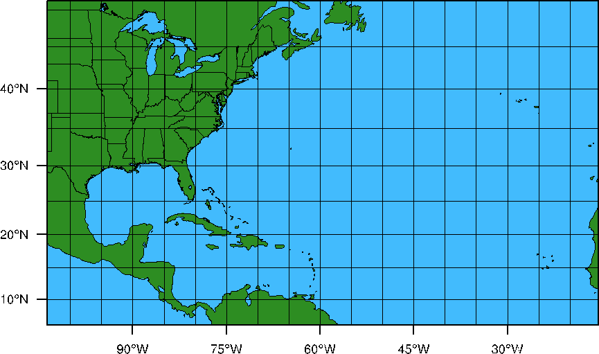
  We are going to create a single domain over North America and the North Atlantic.
  The domain size will be 110x65 grid points, with a grid resolution of 90km. We will use a Mercator projection. (Note: downscaled climate simulations will typically be at a higher resolution than 90km, but since this is just a test case, and we would like to cover a large area, we compromised on the resolution)
   
  • Make the following changes to the namelist:

    max_dom = 1,
    e_we = 110,
    e_sn = 65,
    dx = 90000,
    dy = 90000,
    map_proj = 'mercator',
    ref_lat = 30.00
    ref_lon = -60.00
    truelat1 = 0.0,
    truelat2 = 0.0,
    stand_lon = -60.00
    geog_data_path =

  • geo_data_path: Make sure to change the path to the geogrid static input data to point to the location on the classroom machines (as indicated above).  
    
    
  • Some basic descriptions of the namelist variables are available from the OnLine Tutorial page (geogrid ; ungrib ; metgrid)
  • More detailed information is available in Chapter 3 of your ARW User's Guide
     
     
    
• The above domain will look like this:
  
  

  

   

Run geogrid  

Configure the model grid and generate the geographical data file "geo_em.d01.nc" by running the program geogrid.exe:
 
     ./geogrid.exe

 

Run ungrib

Degrib and reformat meteorological data from reanalysis or climate models. In this case, the data come from NCEP-NCAR Reanalysis 2 (NCEP2), and archived SST. We are going to ungrib the two datasets separately.

• FIRST Link the NCEP2 data using the script file link_grib.csh NOTE:The below command is all one line:
   
       ./link_grib.csh    /kumquat/wrfhelp/DATA/NCEP2/flx.ft06.2003070*    /kumquat/wrfhelp/DATA/NCEP2/pgb.anl.2003070*
  
        NOTE: The NCEP2 data are split into 2D (flx) and 3D (pbg) files and we need to link them all in. This is fine to do in one step.
  
   
  
• Link the correct Vtable (the input data for this case is NCEP2, so use the NCEP2 Vtable):
   
       ln -sf  ungrib/Variable_Tables/Vtable.NCEP2   Vtable
   
  
• Make the following changes to the &share section of the namelist to correctly ingest the data for the right times.
   
  

  &share
  start_date = '2003-07-02_00:00:00',
  end_date = '2003-07-03_00:00:00',
  interval_seconds = 21600,

   
• Ungrib the input data by running the program ungrib.exe:
   
       ./ungrib.exe >& log.ungrib
   
       This will create a number of files:
   
            FILE:2003-07-02_00
            FILE:2003-07-02_06
            FILE:2003-07-02_12
            FILE:2003-07-02_18
            FILE:2003-07-03_00

• SECOND, link the SST data using the script file link_grib.csh:
   
       ./link_grib.csh    /kumquat/wrfhelp/DATA/SST/oisst   
  
   
  
• Link the correct Vtable (the input data for this case is SST, so use the SST Vtable):
   
       ln -sf  ungrib/Variable_Tables/Vtable.SST   Vtable
   
  
• Make the following changes to the &share and &ungrib sections of the namelist to correctly ingest the data for the right times.
        NOTE: The interval between the SST data sets is multiple DAYS. We only have SST data for 2003-07-02 & 2003-07-09.
                  We NEED SST data 6 hourly to match the NCEP2 data interval.
                  By using the available SST dates as start and end time, and by setting interval_seconds to 6 hours,
                  we can interpolate our available data to the required 6 hourly intervals.
                  Also note the prefix change - this is so that we do not overwrite the NCEP2 data we just ungribbed.
   
  

  &share
  start_date = '2003-07-02_00:00:00',
  end_date = '2003-07-09_00:00:00',
  interval_seconds = 21600,
  &ungrib
  prefix = 'SST',

   
• Ungrib the input data by running the program ungrib.exe:
   
       ./ungrib.exe >& log.ungrib
   
       This will create a number of files:
   
            SST:2003-07-02_00 to SST:2003-09-03_00 (one file for every 6 hours)
  


 

Run metgrid

Interpolate external model data to your model grid (created by geogrid and ungrib), and create input data for WRF by running the program metgrid.exe:

Before running metgrid.exe, first make the following change to the &metgrid section of the namelist to ensure both FILE and SST files created by ungrib will be used by metgri:

Set the end date back to 2003-07-03
     end_date = '2003-07-03_00:00:00',

Make sure metgrid reads BOTH the ungribbed files created:

&metgrid
fg_name = 'FILE', 'SST'

Now - run metgrid.
   
     ./metgrid.exe >& log.metgrid
 
     This will create a number of files:
 
          met_em.d01.2003-07-02_00:00:00.nc
          met_em.d01.2003-07-02_06:00:00.nc
          met_em.d01.2003-07-02_12:00:00.nc
          met_em.d01.2003-07-02_18:00:00.nc
          met_em.d01.2003-07-03_00:00:00.nc
 
Try the netcdf data browser 'ncview' to quickly examine your data files from 'metgrid.'  

 

Set-up WRF

• Make sure you are in the WRFV3 directory.    
   
   
• cd to directory test/em_real
   
   
• Edit the namelist.input file
   
       &time_comtrol
       run_hours = 24,
       start_year = 2003,
       start_month = 07,
       start_day = 02,
       start_hour = 00,
       end_year = 2003,
       end_month = 07,
       end_day = 03,
       end_hour = 00,
       interval_seconds = 21600,
       input_from_file = .true.,
       history_interval = 180,
       frames_per_outfile = 1,
       restart = .false.,
       restart_interval = 1440, 
     
       &domains
       time_step = 360,
       max_dom = 1,
       e_we = 110,
       e_sn = 65,
       e_vert = 35,
       p_top_requested = 5000,
       num_metgrid_levels = 18,
       num_metgrid_soil_levels = 2,
       dx = 90000,
       dy = 90000,
  
   
  • Set frames_per_outfile to 1 - this will create a new wrfout file for each output time - this is a good option for long runs, as it makes the output more manageable
  • Note that we are creating restart files - for long runs, you will more than likely have to stop and start often, so create restart files at least once a day.
  • Note the large time step - that is because we are running on a 90km domain.
  • Be careful to not use too few vertical levels when doing long simulations, as this could lead to systematic biases. In this case we picked 35 levels.
  • Also note that we set p_top_requested to 50 hPa. First, we can only do so if our input data include this level (which ours does). Secondly, long simulations benefit from a higher model top, so always try to obtain data with a top of at least 10mb.
     
• Now ADD the following to the namelist.input file under the &time_control and &physics sections
   
       &time_control
       auxinput4_inname = "wrflowinp_d<domain>"
       auxinput4_interval = 360,
       io_form_auxinput4 = 2,
   
       &physics
       sst_update = 1,
  
   
  • The addition of these lines will ensure the updating to SST every 6 hours throughout the model simulation.
  • Do not change the syntax for the auxinput4_inname parameter. WRF understand this syntax and will correctly translate that to the correct file name.
     
     
  
  
• To learn more about the namelist variables view the OnLine Tutorial page, or
• For more details, see Chapter 5 of your ARW User's Guide
  
   
   

Run real

• Link the metgrid output data files from WPS to the current directory:
   
       ln -sf ../../../WPS/met_em* .
   
• Run the executable real.exe to produce model initial and lateral boundary files.
   
  If successful, the following input files for wrf will be created, note the addition wrflowinp_d01 file (this file contains the SST information):
   
       wrfbdy_d01
       wrfinput_d01
       wrflowinp_d01
   
  View the log files to ensure the run was successful.
  

 

Run wrf

• Run the executable wrf.exe for a model simulation as normal.
   
  
  

Check your output:

• Check to see what is printed to the log files.
• Tail the log files and look for "SUCCESS COMPLETE WRF".
   
  
• Try the netcdf data browser 'ncview' to examine your wrf output file
   
• Generate graphics with one of the supplied packages.
   
  

Organization Suggestion:

Recall the suggestion (from the "basic" case) to create a directory to put your files in. Do this again for this case:

mkdir climate_run

and then copy the necessary files into that directory to preserve them for potential later use.

If this was successful, you can continue to run another practical example.