The purpose of this exercise is to familiarize yourself with the basic process of running WRF. The namelists have been modified exactly as they should be for this simple case, so you should not need to make any modifications.
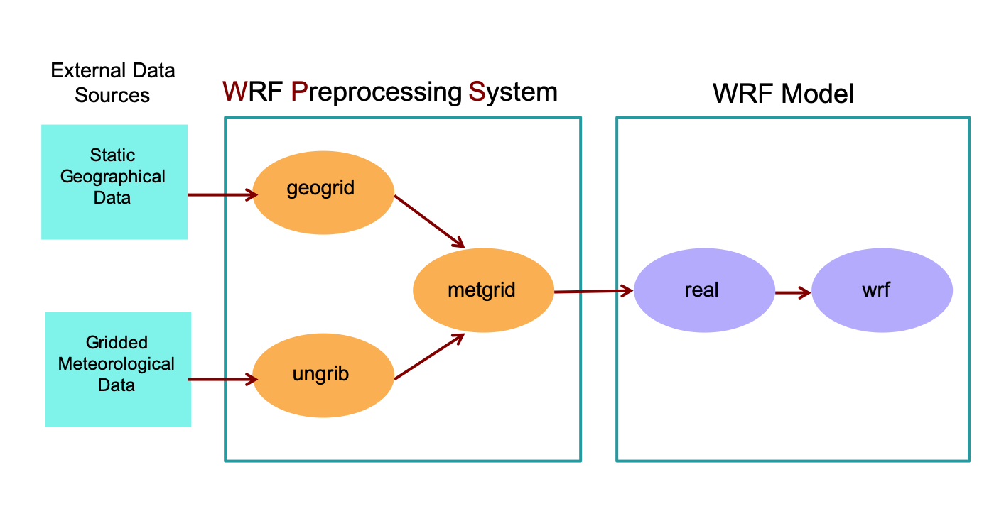
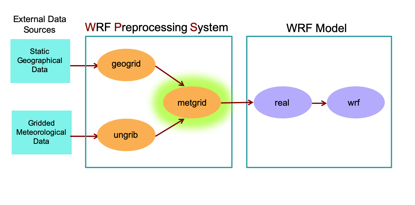
There are 5 steps to running WRF, broken down into 2 major programs: The WRF Preprocessing System (WPS) and the WRF model.
The WPS is a set of three programs that prepare input for the WRF program:
geogrid: defines the model domain and interpolates static geographical data to the grids ungrib: extracts meteorological fields from GRIB-formatted input data files metgrid: horizontally interpolates the meteorological fields extracted by ungrib to the model domain defined by geogrid
The WRF model is broken into 2 programs:
real: vertically interpolates the meteorological fields (from WPS) to WRF eta levels wrf: simulates the model run, using all previously-defined settings for the domain, input data, vertical interpolation, physics, and dynamics settings
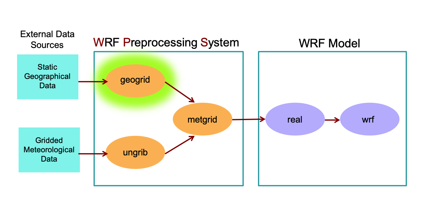
1.
The geogrid program defines the model domain (e.g., map projection, geographic location, size, and resolution of the domain). It also uses static fields (e.g., topography height, landuse category, etc.) from an external source, and interpolates them to the domain.
To run geogrid, you must be in the WPS directory.
cd running/WPS
Typically at this point, you would need to make modifications to the namelist.wps file to define your domain settings, but for this exercise, we have already done this for you!
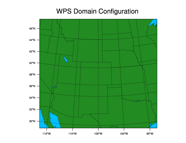
Before running the geogrid.exe program, let's take a look at the domain. You can use a program called plotgrids.ncl to do this.
In the command line, type:
ncl util/plotgrids.ncl
You should see the following plot appear on the screen:
To close the X11 display window, simply click on the image, or type 'ctrl-c'.
Now Configure the model grid by running the program geogrid.exe:
./geogrid.exe
If the run was successful, you will see a "Successful completion of geogrid" message at the end of the print out. You should also now see the following file in your WPS directory:
geo_em.d01.nc
Notes:
You may see a message that says "Optional fields not processed by geogrid" with a list of fields below it. That's ok! These are optional fields and we do not want to process these at this time.
If you would like to take a look at all the fields in the geo_em.d01.nc file, use the ncview tool:
ncview geo_em.d01.nc
To quit ncview, simply type "ctrl-c", or click on the "quit" button.
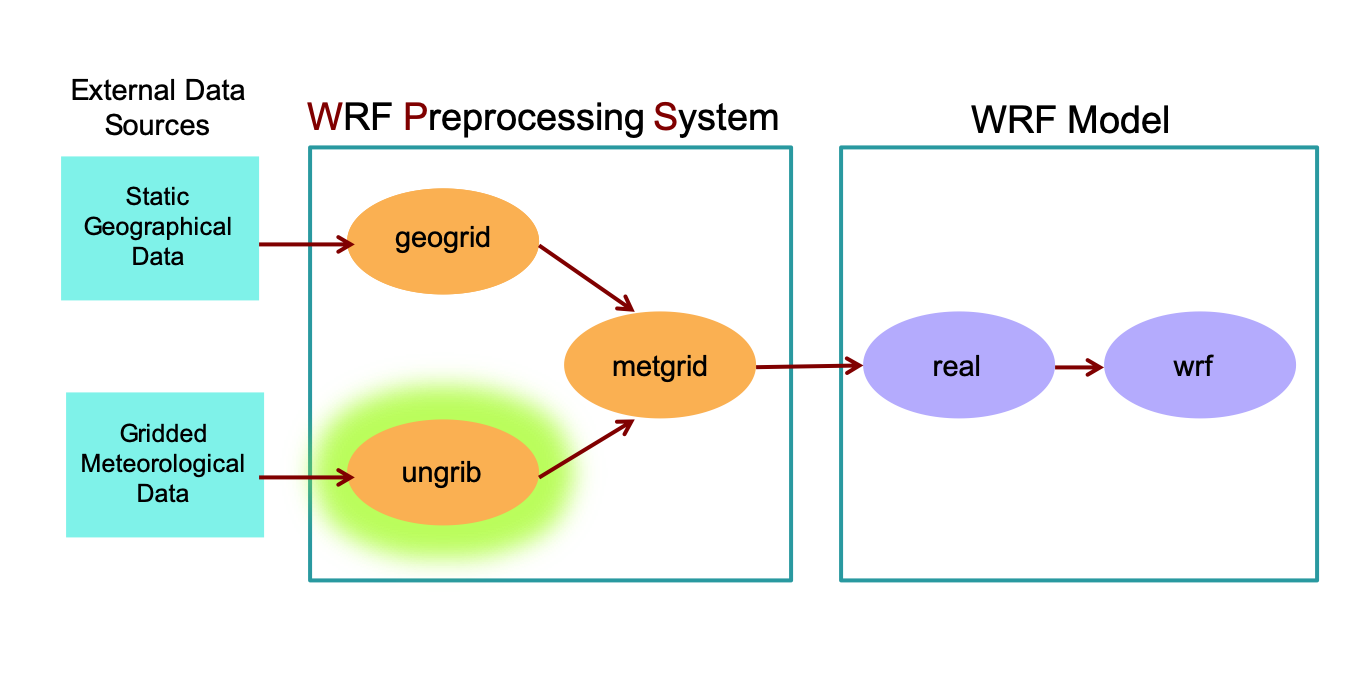
2.
Typically, input data from other models is provided in Grib format. The ungrib program reads these data, extracts the meteorological fields, and then writes those fields to an intermediate file format, so that it can be read by the next program (metgrid).
Our case is a severe snow storm event over Colorado and the data we are using come from the GFS model (FNL: final analysis data: 1 degree resolution), which are 6-hourly data. The data files are stored in the /home/ec2-user/input_data/Colorado directory in your instance.
Again, we have already made essential modifications to the namelist, so you will not need to modify it at this time.
Link the GRIB data into the current directory using the script file "link_grib.csh":
There is no "."
at the end of this command, as this is a script that is
run.
Take care to link to FILES and not to a DIRECTORY.
Only the root section of all the files is needed, and not a list of independent files; therefore,
once you have typed through the name of the directory that holds the grib files, simply hit the 'tab' button
and auto-complete will provide the prefix of the files, which is all that is necessary.
Now if you use the following command:
ls -l GRIB*
you should now see the following GRIB* files, linked to their corresponding input data file (one for each time period):
Note:
The GRIBFILE.XXX formatted name is expected by the ungrib.exe program.
Link the correct Vtable (the input data
for this case is GFS (FNL), so use the GFS Vtable). Vtables are used to determine which fields are necessary to extract from a grib file (as not all fields are needed) and to decode the grib data and convert the files to intermediate format, used as input to the metgrid program. Here you are linking the correct Vtable to this directory and renaming it a generic name 'Vtable' so that the ungrib.exe process will recognize it for processing.
ln
-sf ungrib/Variable_Tables/Vtable.GFS Vtable
Ungrib the input data by running program ungrib.exe:
./ungrib.exe
If the run was successful, you will see a "Successful completion of ungrib" message at the end of the print out, and the following files should have been created in the WPS directory:
These files are now in intermediate format and are ready for the metgrid.exe process.
3.
The metgrid program horizontally interpolates meteorological data (extracted by the ungrib program) to the simulation domains (defined by geogrid). This program will combine the domain information with the meteorological data to create new files that will be used to run the WRF model.
To run the metgrid program, simply type:
./metgrid.exe
If the metgrid.exe process is successful, you will see the message "Successful completion of metgrid" at the end of the print out. And if you issue:
Note: If you would like to take a look at all the fields in the met_em* files, use the ncview tool:
ncview met_em.d01*
To quit ncview, simply type "ctrl-c", or click on the "quit" button.
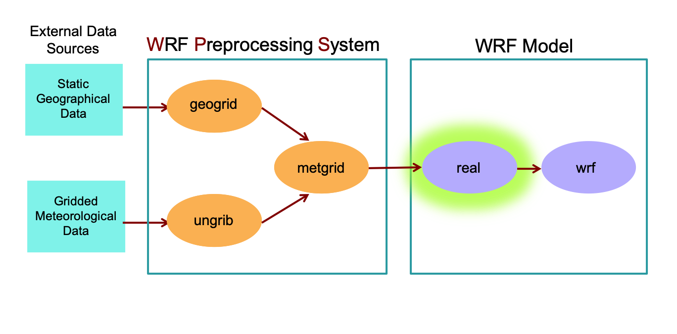
4.
The real program defines the WRF model vertical coordinate. It uses the horizontally-interpolated meteorological data (met_em* files from WPS) and vertically interpolates them for use with the WRF model. It creates initial condition files and a lateral boundary file that will be used by WRF.
To run the real.exe and wrf.exe programs, you need to move to move to the WRF/test/em_real directory. From WPS/, type:
cd ../WRF/test/em_real
Link the metgrid output data
files from WPS to the current directory:
ln -sf ../../../WPS/met_em* .
Typically at this point, you would need to make modifications to the namelist.input file specify the domain, dates, physics options, etc.; however, as the namelist has already been prepared for this exercise, simply run the executable "real.exe" (which uses the met_em* files as input)
to produce model initial and lateral boundary files:
./real.exe
If successful
the following input files for wrf will be created:
wrfbdy_d01
wrfinput_d01
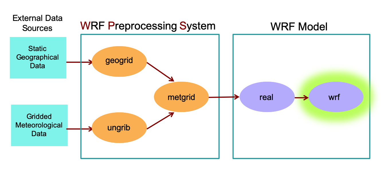
3.
The WRF model uses the intitial and boundary condition files generated by the real program to perform model integration, using user-specified options provided in the namelist.input file (e.g., physics options).
Run the executable "wrf.exe"
for a model simulation and forecast:
mpirun -np 8 ./wrf.exe
Note: Running a 24–hour simulation for this case will take several minutes to complete. Placing the '&' at the end of the command will put this run in the background. If you press the space bar once, you will regain foreground control. To check the status of your run at any time, use the command:
tail rsl.error.0000
When it has completed, you will see a 'SUCCESS' message at the end.
If successful, this will
generate the following history files (we specified in the namelist.input file to output every 3 hours):
If you are interested in viewing some of your output, try the NetCDF data browser "ncview" to examine your wrf output files.
ncview wrfout_d01*
Note:
All output fields will be available to view. You can choose one field at a time to view, and then can click through different time periods and, if the variables are in the 4d column, you can also look at each level. Fields that are 2–dimensional will be listed under the 3D Vars and fields that are 3–dimensional will be listed under the 4D Vars, as they all have a time dimension included. Some particular fields you may be interested in are:
RAINC: Accumulated total cumulus precipitation (under the list of "3d vars") RAINNC: Accumulated total grid scale precipitation (3d) SNOWC: Snow coverage (3d) SNOWNC: Accumulated total grid scale snow and ice (3d) PSFC: Surface pressure (3d) Q2/T2: Water Vapor/Temperature at 2m above ground (3d) U10/V10: X/Y Component of wind (speed) at 10m above ground (3d) MU: Perturbation dry air mass in column (3d) PH: Perturbation geopotentail (under the list of "4d vars") QVAPOR/QCLOUD/QRAIN/QICE/QSNOW: Vapor/Cloud water/Rain water/Ice/Snow mixing ratio (4d) U/V: X/Y-wind component (speed) (4d)
Feel free to also try either the NCL or RIP post-processing programs for plotting output.
Click here to go back to the WRF in the Cloud home page.