Introduction

Tracer advection models the transport of atmospheric constituent fields called tracers, species, or scalars (meaning they are single-value, not a vector field like wind velocity) under the forcing of the wind fields forecast by the WRF model Runge-Kutta dynamics (Skamarock et al. 2008). Examples of tracers in WRF include concentrations of various types of moisture found in the atmosphere (vapor, cloud, rain, etc.), chemical concentrations (e.g. pollutants, reactive species in a wildfire, etc.), or other 3-dimensional fields.

Tracer advection for this benchmark is the WRF 5^th order positive-definite advection scheme (Wicker and Skamarock, 2005). Advection is called once for each Runge-Kutta iteration in the WRF solver. It is a split scheme, advecting each dimension of the domain separately and using finite-difference approximation to compute adjustments, or “tendencies”, that are later applied as updates to each grid cell of each field. Positive definiteness, which prevents negative concentrations, is enforced conservatively and monotonically as an adjustment at the end of the advection scheme (Skamarock and Weisman, 2008). The tracer fields and their tendencies in WRF are organized in 4-dimensional tracer-arrays, the outer index of which is over the tracers, allowing them to be advected and diffused en-masse in a loop over this outer index.

Cost of tracer advection scales linearly with the number of tracers. Advection of five moisture tracers in a typical WRF run accounts for about ten-percent of total run time on a single processor. However, with atmospheric chemistry turned on, the number of tracers is an order of magnitude larger – 81 fields for the test case in this benchmark. Because of this large number of tracers, advection dominates the WRF meteorology’s contribution to the cost of WRF-Chem simulation; however, the additional cost of the chemistry module is a factor of 6 greater than the cost the weather model that drives it (see WRF Chem GPU benchmark page).

Methodology

WRF-Chem was configured to run a large case: 27km resolution 134x110x35 grid over the Eastern U.S. that was part of a large air-quality field campaign in 2006. The input to the RK_SCALAR_TEND routine in the WRF ARW solver was written out at each time step, generating a series of sample input files for the standalone benchmark. The inputs include current and previous RK step values for the 81 chemical tracers in the case, wind velocities, density, and other 3- and 2-dimensional inputs. The call tree rooted at RK_SCALAR_TEND was then extracted from the WRF code and called within a small driver, producing a standalone benchmark driver for the original Fortran, or “vanilla” version of the scalar advection module. Once this was completed, the RK_SCALAR_TEND call tree was converted to C, then CUDA, then optimized for the GPU, and included in the benchmark distribution (below) as the “chocolate” version of the code.

Details of CUDA implementation

Tracer advection has several characteristics that make getting good performance more difficult compared decomposition with the cloud microphysics kernel:

Computational intensity is much lower: only 0.76 floating point operations per memory access compared with 2.2 for microphysics,
Unlike microphysics, there are data-dependencies between threads in a thread-per-column decomposition, because of the 5^th order finite difference stencil width, and
Data transfer of 3-dimensional tracer fields between CPU-GPU.

One the plus-side, there are potentially many tracers to be advected and ample opportunity for overlapping CPU-GPU data transfers with computation using double buffering an asynchronous forms of CUDA calls and kernel invocations. The final CUDA implementation of scalar advection uses textures, a mechanism from graphics that can be used to cache caching multi-dimensional normally high-latency device memory accesses in the shape of the stencil. In CUDA version 1, these textures could be only 2-dimensional and the first versions of this scalar advection scheme had to slice and double-buffer the domain into 2-D slabs. With CUDA version 2, there is now also 3-dimensional texturing, simplifying the code and reducing the number of kernel invocations and data transfer operations by a factor of n.

A final improvement in performance was made by using ‘pinned’ memory on the host side, which increases the speed of CPU-GPU transfers and improves the CUDA implementation of scalar advection by a factor of 1.25 . Pinning can be enabled or disabled in the benchmark code by defining or not defining –DPINNING in the makefile [note: turning off pinning doesn’t work in the current benchmark code]. For more information on pinning in CUDA, see here and the CUDA manuals.

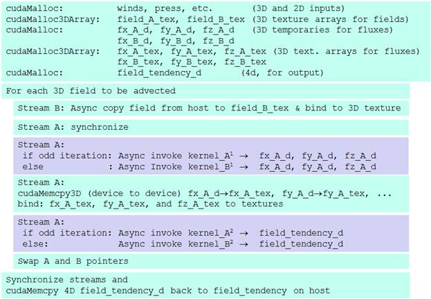
The diagram below shows the steps involved in the GPU implementation of tracer advection. Light aquamarine blocks are executed on the CPU, the lavender blocks are kernel invocations on the GPU. Since it is necessary to synchronize between steps, the full positive-definite tracer advection involves several kernels.

Two sets of textures are needed for double buffering. Curiously and somewhat inconveniently, because textures are defined at compile time in CUDA, it is not possible to switch between them at run-time. This meant that two identical sets of kernel routines (indicated with superscripts in diagram) had to be coded, differing only in name and in which set of textures, A or B, they accessed. This was handled in the benchmark code using macros to autogenerate the two routines from templates.

Results

The benchmark code was tested for the 81-tracer WRF-Chem case a workstation with the following characteristics.

* 2.83 GHz Intel Xeon E5440 quad-core

* Tesla C1060 GPU, 1.296 GHz

* PCIe-2

* Intel Fortran 10.1 (using -O3 -fpe0 optimization)

* Cuda compilation tools, release 2.1, V0.2.1221 (Nov 25th build).

The original “vanilla” Fortran version of the scalar advection ran in 4 seconds. The CUDA version of the code ran in 0.6 seconds, a 6.7x improvement.

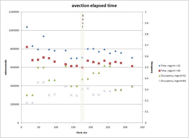
GPU Performance Tuning. As with other kernels tested, performance of the scalar advection code appears to depend most closely on warp occupancy (the number of thread-warps that are actively running on the GPU, which can be measured using the GPU hardware counters available under the CUDA profiling tools). As shown in the figure below, for a particular domain, warp occupancy and ultimately performance are sensitive to GPU-specific tuning parameters such as thread-block size and the number of registers. Optimizing benchmark codes involves sweeps over these controllable parameters.

Output Verification. The output from the two codes (both running single precision) agrees to within %0.1 percent, according to the output verification test included with the benchmark. The test is calculated as follows: for each 3-dimensional field, a mean over cell values in each horizontal (x and y) level is computed and output at the end of the run. Once both the CPU and GPU versions of the code has run, variances of the form |(mean_cpu-mean_gpu)/mean_cpu)| are computed for each pair of means. The output of the test is the arithmetic mean of these variances.

Benchmark code and instructions

The downloadable version of the code contains the driver, the original and CUDA versions of the code, and a README file. Input dataset for the benchmark is very large (>200 MB gzipped) and is downloaded separately.

References

Skamarock, W.C. et al. A Description of the Advaced Research WRF Version 3. NCAR Technical note NCAR/TN-475+STR, June 2008. (pdf)
Skamarock, W. C. and M. L. Weisman, 2008: The impact of positive-definite moisture transport on NWP precipitation forecasts, Mon. Wea. Rev.: submitted.
Wicker, L. J. and W. C. Skamarock, 2002: Time splitting methods for elastic models using forward time schemes, Mon. Wea. Rev., 130, 2088–2097.

Last updated, February 25, 2009 michalak@ucar.edu http://www.mmm.ucar.edu/people/michalakes