User’s Guide for Advanced Research WRF (ARW) Modeling System Version 2
Chapter 5: WRF Model
Table of Contents
- Introduction
- Software Requirement
- Before You Start
- How to Compile WRF?
- How to Run WRF?
- Idealized Case
- Real Data Case
- Restart Run
- One-way and Two-Way Nested Forecasts
- One-Way Nested Forecast Using ndown
- Moving Nest
- Three-dimensional Analysis Nudging
- Observation Nudging
- Check Output
- Physics and Diffusion Options
- Description of Namelist Variables
- List of Fields in WRF Output
Introduction
The WRF model is a fully compressible, and nonhydrostatic model (with a hydrostatic option). Its vertical coordinate is a terrain-following hydrostatic pressure coordinate. The grid staggering is the Arakawa C-grid. The model uses the Runge-Kutta 2nd and 3rd order time integration schemes, and 2nd to 6th order advection schemes in both horizontal and vertical directions. It uses a time-split small step for acoustic and gravity-wave modes. The dynamics conserves scalar variables.
The WRF model code contains several initialization programs (ideal.exe and real.exe; see Chapter 4), a numerical integration program (wrf.exe), and a program to do one-way nesting (ndown.exe). The WRF model Version 2.2 supports a variety of capabilities. These include
· Real-data and idealized simulations
· Various lateral boundary condition options for real-data and idealized simulations
· Full physics options
· Positive-definite advection scheme
· Non-hydrostatic and hydrostatic (runtime option)
· One-way, two-way nesting and moving nest
· Three-dimensional analysis nudging
· Observation nudging
Software requirement
· Fortran 90 or 95 and c compiler
· perl 5.04 or better
· If MPI and OpenMP compilation is desired, it requires MPI or OpenMP libraries
· WRF I/O API supports netCDF, PHD5 and GriB 1/2 formats, hence one of these libraries needs to be available on the computer where you compile and run WRF
Before you start
Before you compile WRF code on your computer, check to see if you have netCDF library installed. This is because one of the supported WRF I/O is netCDF format. If your netCDF is installed in some odd place (e.g. not in your /usr/local/), then you need to know the paths to the netCDF library, and to it’s include/ directory. You may use the environment variable NETCDF to define where the path to netCDF library is. To do so, type
setenv
NETCDF/path-to-netcdf-library
If you don't have netCDF on your computer, you need to install it first. You may download netCDF source code or pre-built binary. Installation instruction can be found on the Unidata Web page athttp://www.unidata.ucar.edu/.
Hint: for Linux users:
If you use PGI or Intel compiler on a Linux computer, make sure your netCDF is installed using the same compiler. Use NETCDF environment variable to point to the PGI/Intel compiled netCDF library.
Hint: NCAR IBM users:
On the other NCAR’s IBM, bluevista and blueice, the netCDF is installed in the ‘usual’ location, /usr/local, and only the 64-bit libraries are installed. No need to set anything prior to compilation.
How to compile WRF?
WRF source code tar file may be downloaded from http://www2.mmm.ucar.edu/wrf/download/get_source.html. Once you obtain the tar file, gunzip, and untar the file, and this will create a WRFV2/ directory. This contains:
|
Makefile |
Top-level makefile |
|
README |
General information about WRF code |
|
README_test_cases |
Explanation of the test cases |
|
Registry/ |
Directory for WRF Registry file |
|
arch/ |
Directory where compile options are gathered |
|
clean |
script to clean created files, executables |
|
compile |
script for compiling WRF code |
|
configure |
script to configure the configure.wrf file for compile |
|
chem/ |
Developer code, not yet supported |
|
dyn_em/ |
Directory for modules for dynamics in current WRF core (Advanced Research WRF core) |
|
dyn_exp/ |
Directory for a 'toy' dynamic core |
|
dyn_nmm/ |
NCEP NMM core, supported by DTC |
|
external/ |
Directory that contains external packages, such as those for IO, time keeping and MPI |
|
frame/ |
Directory that contains modules for WRF framework |
|
inc/ |
Directory that contains include files |
|
main/ |
Directory for main routines, such as wrf.F, and all executables after compilation |
|
phys/ |
Directory for all physics modules |
|
run/ |
Directory where one may run WRF |
|
share/ |
Directory that contains mostly modules for WRF mediation layer and WRF I/O |
|
test/ |
Directory that contains 7 test case directories, may be used to run WRF |
|
tools/ |
Directory that contains tools for |
Go to WRFV2 (top) directory.
Type
configure,
or ./configure
and you will be given a list of choices for your computer. These choices range from compiling for a single processor job, to using OpenMP shared-memory or distributed-memory parallelization options for multiple processors. Some options support nesting, others do not. Some use RSL-LITE, others use RSL. So select the option carefully. For example, the choices for a Linux computer looks like this:
checking for perl5... no
checking for perl... found /usr/bin/perl (perl)
Will use NETCDF in dir: /usr/local/netcdf-pgi
PHDF5 not set in environment. Will configure WRF for use without.
------------------------------------------------------------------------ Please select from among the following supported platforms.
1. PC Linux i486 i586
i686,PGI compiler (Single-threaded, no nesting)
2. PC Linux i486 i586 i686, PGI compiler (single threaded, allows nesting using
RSL without MPI)
3. PC Linux i486 i586 i686, PGI compiler SM-Parallel (OpenMP, no nesting)
4. PC Linux i486 i586 i686, PGI compiler SM-Parallel (OpenMP, allows nesting
using RSL without MPI)
5. PC Linux i486 i586 i686, PGI compiler DM-Parallel (RSL, MPICH, Allows
nesting)
6. PC Linux i486 i586 i686, PGI compiler DM-Parallel (RSL_LITE, MPICH, Allows
nesting)
7. Intel xeon i686 ia32 Xeon Linux, ifort compiler (single-threaded, no
nesting)
8. Intel xeon i686 ia32 Xeon Linux, ifort compiler (single threaded, allows
nesting using RSL without MPI)
9. Intel xeon i686 ia32 Xeon Linux, ifort compiler (OpenMP)
10. Intel xeon i686 ia32 Xeon Linux, ifort compiler SM-Parallel (OpenMP, allows
nesting using RSL without MPI)
11. Intel xeon i686 ia32 Xeon Linux, ifort+icc compiler DM-Parallel (RSL,MPICH,
allows nesting)
12. Intel xeon i686 ia32 Xeon Linux, ifort+gcc compiler DM-Parallel (RSL,MPICH,
allows nesting)
13. PC Linux i486 i586 i686, PGI compiler, ESMF (Single-threaded, ESMF
coupling, no nesting)
Enter
selection[1-13] :
Enter a number for an option that is best for your computer and application.
You will see a configure.wrf file created. Edit compile options/paths, if necessary.
Hint: for choosing RSL_LITE versus RSL:
Choose compile options that use RSL_LITE whenever one can. The only option RSL_LITE doesn’t support is the periodic boundary condition in y. RSL_LITE is a bit faster, and will work for domains dimensioned greater than 1024x1024. The positive-definite advection scheme is implemented using RSL_LITE only.
Hint: for nesting compile:
On most platforms, this requires RSL_LITE or RSL, even if you only have one processor. Check the options carefully and select those which support nesting.
Hint: On some computers (e.g. some Intel machines), it may be necessary to set the following environment variable before one compiles:
setenv WRF_EM_CORE 1
Type 'compile', or ‘./compile’ and it will show the choices:
Usage:compile wrf compile wrf in run dir (Note, no real.exe, ndown.exe or ideal.exe generated)test cases (see README_test_cases for details):
compile em_b_wavecompile em_grav2d_xcompile em_hill2d_xcompile em_quarter_sscompile em_realcompile em_squall2d_xcompile em_squall2d_y
compile –h help messagewhere em stands for the Advanced Research WRF dynamic solver (which currently is the 'Eulerian mass-coordinate' solver). Type one of the above to compile. When you switch from one test case to another, you must type one of the above to recompile. The recompile is necessary to create a new initialization executable (i.e. real.exe, and ideal.exe - there is a different ideal.exe for each of the idealized test cases), while wrf.exe is the same for all test cases.
If you want to remove all object files (except those in external/directory) and executables, type 'clean'.
Type 'clean -a' to remove built files in ALL directories, including configure.wrf. This is recommended if you make any mistake during the process, or if you have edited the Registry.EM file.
a. Idealized case
Type 'compile case_name' to compile. Suppose you would like to run the2-dimensional squall case, type
compile em_squall2d_x
or
compile
em_squall2d_x>& compile.log
After a successful compilation, you should have two executables created in the main/directory: ideal.exe and wrf.exe. These two executables will be linked to the corresponding test/ and run/directories. cd to either directory to run the model.
b. Real-data case
Compile WRF model after 'configure', type
compile em_real
or
compile em_real >& compile.log
When the compile is successful, it will create three executables in the main/directory: ndown.exe, real.exe and wrf.exe.
real.exe:
for WRF initialization of real data cases
ndown.exe
: for one-way nesting
wrf.exe
: WRF model integration
Like
in the idealized cases, these executables will be linked to test/em_real
and run/
directories. cd
to one of these two directories to run the model.
How to run WRF?
After a successful compilation, it is time to run the model. You can do so by either cd to the run/ directory, or the test/case_name directory. In either case, you should see executables, ideal.exe or real.exe, and wrf.exe, linked files(mostly for real-data cases), and one or more namelist.input files in the directory.
Idealized, real data, restart run, two-way nested, and one-way nested runs are explained on the following pages. Read on.
Suppose you choose to compile the test case em_squall2d_x, now type 'cd test/em_squall2d_x'or 'cd run' to go to a working directory.
Edit namelist.input file (see README.namelist in WRFV2/run/ directory or its Web version) to change length of integration, frequency of output, size of domain, timestep, physics options, and other parameters.
If you see a script in the test case directory, called run_me_first.csh, run this one first by typing:
run_me_first.csh
This links some data files that you might need to run the case.
To run the initialization program, type
ideal.exe
This will generate wrfinput_d01 file in the same directory. All idealized cases do not require lateral boundary file because of the boundary condition choices they use, such as the periodic boundary condition option.
Note:
- ideal.exe cannot generally be run in parallel. For parallel compiles, run this on a single processor.
- The exception is the quarter_ss case, which can now be run in MPI.
To run the model, type
wrf.exe
or variations such as
wrf.exe >& wrf.out
&
Note:
- Two-dimensional ideal cases cannot be run in MPI parallel. OpenMP is ok.
- The execution command may be different for MPI runs on different machines, e.g. mpirun.
After successful completion, you should see wrfout_d01_0001-01-01* and wrfrst* files, depending on how one specifies the namelist variables for output.
Type 'cd test/em_real' or 'cd run', and this is where you are going to run both the WRF initialization program, real.exe, and WRF model, wrf.exe. Start with a namelist.input file template in the directory, edit it to fit your case.
-
Running real.exe using WPS output
Running a real-data case requires successfully running the WRF Preprocessing System programs(or WPS) and make sure met_em.* files from WPS are seen in the run directory. Make sure you edit the following variables in namelist.input file:
num_metgrid_levels:
number of_ incoming data levels (can be found by using ncdump command on
met_em.d01.<date> file)
eta_levels:
model eta levels from 1 to 0, if you choose to do so. If not, real will compute
a nice set of eta levels for you.
Other options for use to assist vertical interpolation are:
force_sfc_in_vinterp: force vertical
interpolation to use surface data
lowest_lev_from_sfc: place surface
data in the lowest model level
p_top_requested: pressure top used in
the model, default is 5000 Pa
interp_type: vertical interpolation
method: linear in p(default) or log(p)
lagrange_order: vertical
interpolation order, linear (default) or quadratic
zap_close_levels: allow surface data
to be used if it is close to a constant pressure level.
-
Running real.exe using SI output
Running a real-data case requires successfully running the WRF Standard
Initialization program. Make sure wrf_real_input_em.* files
from the Standard Initialization are in this directory (you may link the files
to this directory).
If you use SI, you must use the SI version 2.0 and
above, to prepare input for V2 WRF! Make sure you also have this line in your
namelist.input file (the default input file is expected to come from WPS):
auxinput1_inname = “wrf_real_input_em.d<domain>.<date>”
For both WPS and SI output, edit namelist.input for start and end dates, and domain dimensions. Also edit time step, output, nest and physics options.
Type 'real.exe' to produce wrfinput_d01 and wrfbdy_d01 files. In real data case, both files are required.
Run
WRF model by typing
wrf.exe
A successful run should produce one or several output files named like wrfout_d01_yyyy-mm-dd_hh:mm:ss.For example, if you start the model at 1200 UTC, January 24 2000, then your first output file should have the name:
wrfout_d01_2000-01-24_12:
It is always good to check the times written to the output file by typing:
ncdump -v Times wrfout_d01_2000-01-24_12:
You may have other wrfout files depending on the namelist options (how often you split the output files and so on using namelist option frames_per_outfile).You may also create restart files if you have restart frequency (restart_interval in the namelist.input file) set within your total integration length. The restart file should have names like
wrfrst_d01_yyyy-mm-dd_hh:mm:ss
For DM (distributed memory) parallel systems, some form of mpirun command will be needed here. For example, on a Linux cluster, the command to run MPI code and using 4 processors may look like:
mpirun -np 4 real.exe
mpirun -np 4 wrf.exe
On some IBMs, the command may be:
poe real.exe
poe wrf.exe
for a batch job, and
poe real.exe -rmpool 1-procs
4
poe wrf.exe -rmpool 1 -procs 4
for
an interactive run. (Interactive MPI job is not an option on the new NCAR IBMs bluevista and blueice)
c. Restart Run
A restart run allows a user to
extend a run to a longer simulation period. It is effectively a continuous run
made of several shorter runs. Hence the results at the end of one or more
restart runs should be identical to a single run without any restart.
In order to do a restart run, one
must first create restart file. This is done by setting namelist variable restart_interval (unit is in minutes) to
be equal to or less than the simulation length, as specified by run_* variables or start_* and end_* times.
When the model reaches the time to write a restart file, a restart file named wrfrst_<domain_id>_<date>
will
be written. The date string represents the time when the restart file is valid.
When one starts the restart run,
edit the namelist.input file, so that
your start_* time will be set to the
restart time (and the time a restart file is written). The other namelist
variable one must set is restart, this variable should be set to
.true. for a restart run.
d. One-way and Two-way Nested Forecasts
WRFV2 supports a two-way nest option in both 3-D idealized cases (quarter_ss and b_wave) and real data cases. The model can handle multiple domains at the same nest level (no overlapping nest), and multiple nest levels (telescoping). A moving nest option has also been available since V2.0.3.1.
Note: By setting the feedback switch in the namelist.input file to 0 or 1, the domains behave as 1-way or 2-way nests, respectively.
Make sure that you compile the code with nest options.
Most of options to start a nest run are handled through the namelist. All variables in the namelist.input file that have multiple columns of entries need to be edited with caution. The following are the key namelist variables to modify:
start_ and end_year/month/day/minute/second: these control the nest start and end times
input_from_file: whether a nest requires an input file (e.g. wrfinput_d02). This is typically an option for a real data case.
fine_input_stream: which fields from the nest input file are used in nest initialization. The fields to be used are defined in the Registry.EM. Typically they include static fields (such as terrain, landuse), and masked surface fields (such as skintemp, soil moisture and temperature).
max_dom: setting this to a number > 1 will invoke nesting. For example, if you want to have one coarse domain and one nest, set this variable to 2.
grid_id: domain identifier will be used in the wrfout naming convention.
parent_id:use the grid_id to define the parent_id number for a nest. The most coarse grid must be grid_id = 1.
i_parent_start/j_parent_start: lower-left corner starting indices of the nest domain in its parent domain. These parameters should be the same in namelist.wps, if you use WPS. (If you use SI, you should find these numbers in your SI's $MOAD_DATAROOT/static/wrfsi.nl, namelist file, and look for values in the second(and third, and so on) column of DOMAIN_ORIGIN_LLI and DOMAIN_ORIGIN_LLJ).
parent_grid_ratio: integer parent-to-nest domain grid size ratio. If feedback is off, then this ratio can be even or odd. If feedback is on, then this ratio has to be odd.
parent_time_step_ratio: time ratio for the coarse and nest domains may be different from the parent_grid_ratio. For example, you may run a coarse domain at 30 km, and a nest at 10 km, the parent_grid_ratio in this case is 3. But you do not have to use 180 sec for the coarse domain and 60 for the nest domain. You may use, for example, 45 sec or90 sec for the nest domain by setting this variable to 4 or 2.
feedback: this option takes the values of prognostic variables (average of cell for mass points, and average of the cell face for horizontal momentum points) in the nest and overwrites the values in the coarse domain at the coincident points. This is the reason currently that it requires odd parent_grid_ratio with this option.
smooth_option: this a smoothing option for the parent domain if feedback is on. Three options are available: 0 = no smoothing; 1 = 1-2-1 smoothing; 2 =smoothing-desmoothing. (There was a bug for this option in pre-V2.1 code, and it has been fixed.)
3-D Idealized Cases
For3-D idealized cases, no additional input files are required. The key here is the specification of the namelist.input file. What the model does is to interpolate all variables required in the nest from the coarse domain fields. Set
input_from_file = F, F
Real Data Cases
For real-data cases, three input options are supported. The first one is similar to running the idealized cases. That is to have all fields for the nest interpolated from the coarse domain (namelist variable input_from_file set to F for each domain). The disadvantage of this option is obvious, one will not benefit from the higher resolution static fields (such as terrain, landuse, and so on).
The second option is to set input_from_file = T for each domain, which means that the nest will have a nested wrfinput file to read in (similar to MM5 nest option IOVERW = 1). The limitation of this option is that this only allows the nest to start at hour 0 of the coarse domain run.
The third option is in addition to setting input_from_file = T for each domain, also set fine_input_stream = 2 for each domain. Why a value of 2? This is based on current Registry setting which designates certain fields to be read in from auxiliary input stream 2. This option allows the nest initialization to use 3-D meteorological fields interpolated from the coarse domain, static fields and masked, time-varying surface fields from nest wrfinput. It hence allows a nest to start at a later time than hour 0. Setting fine_input_stream = 0 is equivalent to the second option. This option was introduced in V2.1.
To run real.exe for a nested run, one must first run WPS (or SI) and create data for all the nests. Suppose one has run WPS for a two-domain nest case, and created these files in a WPS directory:
met_em.d01.2000-01-24_12:00:00
met_em.d01.2000-01-24_18:00:00
met_em.d01.2000-01-25_00:00:00
met_em.d01.2000-01-25_06:00:00
met_em.d01.2000-01-25_12:00:00
met_em.d02.2000-01-24_12:00:00
Link
or move all these files to the run directory, which could be run/ or em_real/.
Edit the namelist.input file and set the correct values for all relevant variables, described in the previous pages (in particular, set max_dom = 2,_ for the total number of nests one wishes to run, and num_metgrid_levels for number of incoming data levels),as well as physics options. Type the following to run:
real.exe
or
mpirun –np 4 real.exe
If successful, this will create all input files for coarse as well as nest domains. For a two-domain example, these are
wrfinput_d01
wrfinput_d02
wrfbdy_d01
The way to create nested input files has been greatly simplified due to some improvement introduced to WRF Version 2.1.2 (released in January 2006).
To run WRF, type
wrf.exe
or
mpirun –np 4 wrf.exe
If successful, the model should create wrfout files for both domain 1 and 2:
wrfout_d01_2000-01-24_12:00:00
wrfout_d02_2000-01-24_12:
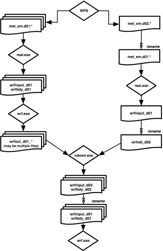
e. One-way Nested Forecast Using ndown
WRF supports two separate one-way nested option. In this section, one-way nesting is defined as a finer-grid-resolution run made as a subsequent run after the coarser-grid-resolution run, where the ndown program is run in between the two forecasts. The initial and lateral boundary conditions for this finer-grid run are obtained from the coarse grid run, together with input from higher resolution terrestrial fields (e.g. terrain, landuse, etc.), and masked surface fields (such as soil temperature and moisture). The program that performs this task is ndown.exe. Note that the use of this program requires that the code is compiled for nesting.
When one-way nesting is used, the coarse-to-fine grid ratio is only restricted to be an integer. An integer less than or equal to 5 is recommended.
To make a one-way nested run involves these steps:
1)
Generate a coarse-grid forecast
2) Make temporary fine-grid initial condition wrfinput_d01 file (note that only
a single time period is required, valid at the desired start time of the
fine-grid domain)
3) Run program ndown, with coarse-grid WRF model
output, and a fine-grid initial condition (to generate fine grid initial and
boundary conditions, similar to the output from the real.exe program)
4)Run the fine-grid forecast
To compile, choose an option that supports nesting.
Step 1: Make a coarse grid run
This is no different than any of the single domain WRF run as described above.
Step 2: Make a temporary fine grid initial condition file
The purpose of this step is to ingest higher resolution terrestrial fields and corresponding land-water masked soil fields.
Before doing this step, one would have run WPS (or SI) and requested one coarse and one nest domain, and for the one time period one wants to start the one-way nested run. This generates a WPS output for the nested domain (domain 2) named met_em.d02.* (or wrf_real_input_em.d02.* from SI).
-
Rename met_em.d02.* to met.d01.* for the single requested
fine-grid start time. Move the original domain
1 WPS output files before you do this.
- Edit the namelist.input file for fine-grid domain (pay attention to
column 1 only) and edit in the correct start time, grid dimensions and physics
options.
- Run real.exe for this domain. This will produce a wrfinput_d01 file.
- Rename this wrfinput_d01 file
to wrfndi_d02.
Step 3: Make the final fine-grid initial and boundary condition files
-
Edit namelist.input again, and this time one needs to edit two
columns: one for dimensions of the coarse grid, and one for the fine grid. Note
that the boundary condition frequency (namelist.input
variable interval_seconds) is
the time in seconds between the coarse-grid output times.
- Run ndown.exe,
with inputs from the coarse grid wrfout files, and wrfndi_d02 file generated from Step 2 above.
This will produce wrfinput_d02
and wrfbdy_d02
files.
Note that one may run program ndown with either distributed memory or serially, depending on the selected compiler options. The ndown program must be built to support nesting, however. For example,
mpirun -np 4 ndown.exe
or
ndown.exe
Step 4: Make the fine-grid WRF run
-
Rename wrfinput_d02 and wrfbdy_d02 to wrfinput_d01 and wrfbdy_d01,
respectively.
- Edit namelist.input one more time, and it is now for the fine-grid domain
only.
- Run WRF for this grid.
The following figure summarizes the data flow for a one-way nested run using program ndown.
The moving nest option is supported in the current WRF. Two types of moving tests are allowed. In the first option, a user specifies the nest movement in the namelist. The second option is to move the nest automatically based on an automatic vortex-following algorithm. This option is designed to follow the movement of a well defined tropical cyclone.
To make the specified moving nest runs, one first needs to compile the code with-DMOVE_NESTS flag added to ARCHFLAGS in the configure.wrf file. To run the model, only the coarse grid input files are required. In this option, the nest initialization is defined from the coarse grid data - no nest input is used. In addition to the namelist options applied to a nested run, the following needs to be added to namelist section &domains:
num_moves: the total number of moves one can make in a model run. A move of any domain counts against this total. The maximum is currently set to 50, but it can be changed by change MAX_MOVES in frame/module_driver_constants.F.
move_id: a list of nest IDs, one per move, indicating which domain is to move for a given move.
move_interval: the number of minutes since the beginning of the run that a move is supposed to occur. The nest will move on the next time step after the specified instant of model time has passed.
move_cd_x,move_cd_y:distance in number of grid points and direction of the nest move(positive numbers indicating moving toward east and north, while negative numbers indicating moving toward west and south).
To make the automatic moving nest runs, two compiler flags are needed in ARCHFLAGS: -DMOVE_NESTS and -DVORTEX_CENTER. (Note that this compile would only support auto-moving nest runs, and will not support_ the specified moving nest at the same time.) Again, no nest input is needed. If one wants to use values other than the default ones, add and edit the following namelist variables in &domains section:
vortex_interval: how often the vortex position is calculated in minutes (default is 15 minutes).
max_vortex_speed: used with vortex_interval to compute the radius of search for the new vortex center position (default is 40 m/sec).
corral_dist: the distance in number of coarse grid cells that the moving nest is allowed to come near the coarse grid boundary (default is 8).
In both types of moving nest runs, the initial location of the nest is specified through i_parent_start and j_parent_start in the namelist.input file.
The automatic moving nest works best for well-developed vortex.
g. Three-Dimensional Analysis
Nudging Run
This option is introduced in V2.2.
Prepare input data to WRF as usual
whether you use WPS or SI. If you would like to nudge in the nest domains as
well, make sure you process all time periods for all domains.
Before you run real.exe, set the
following options, in addition to others described earlier (see namelist
template namelist.input.grid_fdda in test/em_real/ directory for guidance):
grid_fdda = 1
Run real.exe as before, and this
will create, in addition to wrfinput_d01 and wrfbdy_d01 files, a file
named“wrffdda_d01” by default. Other grid nudging namelists are ignored at this
stage. But it is a good practice to fill them all before one runs real. In
particular, set
gfdda_inname = “wrffdda_d<domain>”
gfdda_interval = time interval of input data in minutes
gfdda_end_h = end time of grid nudging in hours
See http://www2.mmm.ucar.edu/wrf/users/wrf_files/docs/How_to_run_grid_fdda.html
and README.grid_fdda in WRFV2/test/em_real/ for more information.
h. Observation Nudging Run
This option is introduced in V2.2.
In addition to the usual input data
preparation from running WPS or SI, one needs to prepare an observation files
to be used in the model. See http://www2.mmm.ucar.edu/wrf/users/docs/How_to_run_obs_fdda.html
for instructions. The observation file names expected by WRF are OBS_DOMAIN101 for domain 1, and OBS_DOMAIN201 for domain 2, etc.
Once one has the observation file(s)
prepared, one can activate the observation nudging options in WRF:
obs_nudge_opt = 1
fdda_start = 0 (obs nudging start time in minutes)
fdda_end = 360 (obs nudging end time in minutes)
See http://www2.mmm.ucar.edu/wrf/users/docs/How_to_run_obs_fdda.htmland README.obs_fdda in WRFV2/test/em_real/ for more information.
Check Output
Once a model run is completed, it
is a good practice to check a couple of things quickly.
-
If
you have run the model on multiple processors using MPI, you should have a
number of rsl.out.* and rsl.error.* files. Type ‘tail rsl.out.0000’ to see if you get ‘SUCCESS COMPLETE WRF’. This is a good indication that
the model run successfully.
-
Check
the output times written to wrfout* file by using netCDF command ‘ncdump –v
Times wrfout_d01_yyyy-mm-dd_hh:00:00’.
-
Take
a look at either rsl.out.0000 file or other standard out file you may have created. This
file logs the times taken to compute for one model time step, and to write one
history and restart output:
Timing for main: time 2006-01-21_23:55:00 on domain 2:
4.91110 elapsed seconds.
Timing for main:
time 2006-01-21_23:56:00 on domain
2: 4.73350 elapsed seconds.
Timing for main: time
2006-01-21_23:57:00 on domain 2: 4.72360 elapsed seconds.
Timing for main:
time 2006-01-21_23:57:00 on domain
1: 19.55880 elapsed seconds.
and
Timing for
Writing wrfout_d02_2006-01-22_00:00:00 for domain 2: 1.17970 elapsed seconds.
Timing for main:
time 2006-01-22_00:00:00 on domain 1: 27.66230 elapsed seconds.
Timing for
Writing wrfout_d01_2006-01-22_00:00:00 for domain 1: 0.60250 elapsed seconds.
If the model did not run to
completion, take a look at these standard output/error files too. If the model
has become numerically unstable, it may have violated the CFL criterion. Check
whether this is true by typing the following:
grep cfl
rsl.error.* or grep cfl
wrf.out
you might see something like these:
5 points exceeded
cfl=2 in domain 1 at time 4.200000
MAX AT i,j,k: 123 48 3 cfl,w,d(eta)= 4.165821
21 points
exceeded cfl=2 in domain 1 at
time 4.200000
MAX AT i,j,k:
123 49 4 cfl,w,d(eta)= 10.66290
When
this happens, often reducing time step can help.
Physics and Dynamics Options
Physics Options
WRF offers multiple physics options that can be combined in any way. The options typically range from simple and efficient to sophisticated and more computationally costly, and from newly developed schemes to well tried schemes such as those in current operational models.
The choices vary with each major WRF release, but here we will outline those available in WRF Version 2.2.
1.
Microphysics (mp_physics)
a. Kessler scheme: A warm-rain (i.e. no ice) scheme used commonly in idealized cloud modeling studies (mp_physics = 1).
b. Lin et al. scheme: A sophisticated scheme that has ice, snow and graupel processes, suitable for real-data high-resolution simulations (2).
cowry Single-Moment 3-class scheme: A simple efficient scheme with ice and snow processes suitable for mesoscale grid sizes (3).
d. WRF Single-Moment 5-class scheme: A slightly more sophisticated version of (c)that allows for mixed-phase processes and super-cooled water (4).
e. Eta microphysics: The operational microphysics in NCEP models. A simple efficient scheme with diagnostic mixed-phase processes (5).
f. WRF Single-Moment 6-class scheme: A scheme with ice, snow and graupel processes suitable for high-resolution simulations (6).
g. Thompson et al. scheme: A new scheme with ice, snow and graupel processes suitable for high-resolution simulations (8; replacing the version in 2.1)
h. NCEP 3-class: An older version of (c) (98).
i.
NCEP 5-class: An older version of (d) (99).
2.1
Longwave Radiation (ra_lw_physics)
a. RRTM scheme: Rapid Radiative Transfer Model. An accurate scheme using look-up tables for efficiency. Accounts for multiple bands, trace gases, and microphysics species (ra_lw_physics = 1).
b. GFDL scheme: Eta operational radiation scheme. An older multi-band scheme with carbon dioxide, ozone and microphysics effects (2).
c.
CAM scheme: from the
2.2 Shortwave Radiation (ra_sw_physics)
a. Dudhia scheme: Simple downward integration allowing efficiently for clouds and clear-sky absorption and scattering (ra_sw_physics = 1).
b. Goddard shortwave: Two-stream multi-band scheme with ozone from climatology and cloud effects (2).
c. GFDL shortwave: Eta operational scheme. Two-stream multi-band scheme with ozone from climatology and cloud effects (99).
d.
CAM scheme: from the
3.1 Surface Layer (sf_sfclay_physics)
a.MM5 similarity: Based on Monin-Obukhov with Carslon-Boland viscous sub-layer and standard similarity functions from look-up tables (sf_sfclay_physics = 1).
b. Eta similarity: Used in Eta model. Based on Monin-Obukhov with Zilitinkevich thermal roughness length and standard similarity functions from look-up tables(2).
3.2 Land Surface (sf_surface_physics)
a.5-layer thermal diffusion: Soil temperature only scheme, using five layers (sf_surface_physics = 1).
b. Noah Land Surface Model: Unified NCEP/NCAR/AFWA scheme with soil temperature and moisture in four layers, fractional snow cover and frozen soil physics (2).
-Urban canopy model (ucmcall):3-category UCM option
c.
4. Planetary Boundary layer (bl_pbl_physics)
a.
b. Mellor-Yamada-Janjic scheme: Eta operational scheme. One-dimensional prognostic turbulent kinetic energy scheme with local vertical mixing (2).
c.
MRF scheme: Older version of (a) with implicit treatment of entrainment layer
as part of non-local-K mixed layer (99).
5. Cumulus Parameterization (cu_physics)
a.
Kain-Fritsch scheme: Deep and shallow convection sub-grid scheme using a mass
flux approach with downdrafts and
b. Betts-Miller-Janjic scheme. Operational Eta scheme. Column moist adjustment scheme relaxing towards a well-mixed profile (2).
c. Grell-Devenyi ensemble scheme: Multi-closure, multi-parameter, ensemble method with typically 144 sub-grid members (3).
d.
Old Kain-Fritsch scheme: Deep convection scheme using a mass flux approach with
downdrafts and
Diffusion and Damping Options
Diffusion in WRF is categorized under two parameters, the diffusion option and the K option. The diffusion option selects how the derivatives used in diffusion are calculated, and the K option selects how the K coefficients are calculated. Note that when a PBL option is selected, vertical diffusion is done by the PBL scheme, and not by the diffusion scheme.
1.1 Diffusion Option (diff_opt)
a. Simple diffusion: Gradients are simply taken along coordinate surfaces (diff_opt= 1).
b. Full diffusion: Gradients use full metric terms to more accurately compute horizontal gradients in sloped coordinates (diff_opt = 2).
1.2 K Option (km_opt)
Note that when using a PBL scheme, only options (a) and (d) below make sense, because (b) and (c) are designed for 3d diffusion.
a. Constant: K is specified by namelist values for horizontal and vertical diffusion (km_opt = 1).
b.3d TKE: A prognostic equation for turbulent kinetic energy is used, and K is based on TKE (km_opt = 2).
c.3d Deformation: K is diagnosed from 3d deformation and stability following a Smagorinsky approach (km_opt = 3).
d.2d Deformation: K for horizontal diffusion is diagnosed from just horizontal deformation. The vertical diffusion is assumed to be done by the PBL scheme (km_opt =4).
1.3 6th Order Horizontal Diffusion (diff_6th_opt)
6th-orderhorizontal
hyper diffusion (
2. Damping Options
These are independently activated choices.
a. Upper Damping: Either a layer of increased diffusion or a Rayleigh relaxation layer can be added near the model top to control reflection from the upper boundary.
b.
w-Damping: For operational robustness, vertical motion can be damped to prevent
the model from becoming unstable with locally large vertical
velocities. This only affects strong updraft cores, so has very little impact
on results otherwise.
c. Divergence Damping: Controls horizontally propagating sound waves.
d. External Mode Damping: Controls upper-surface (external) waves.
e.
Time Off-centering (epssm): Controls vertically propagating sound waves.
3. Advection Options
a. Horizontal advection orders for momentum (h_mom_adv_order) and scalar (h_sca_adv_order) can be 2ndto 6th, with 5th order being the recommended one.
b. Vertical advection orders for momentum (v_mom_adv_order) and scalar (v_sca_adv_order) can be 2ndand 6th, with 3rd order being the recommended one.
c. Positive-definite advection option can be applied to moisture (pd_moist= .true.), scalar (pd_scalar), chemistry variables (pd_chem) and tke (pd_tke).
4. Other Dynamics Options
a.
The model can be run hydrostatically by setting non_hydrostatic switch to .false.
b. Coriolis term can be applied to wind perturbation (pert_coriolis = .true.) only (idealized only).
c. For diff_opt = 2 only, vertical
diffusion may act on full fields(not just on perturbation from 1D base profile
(mix_full_fields = .true.; idealized
only).
Description of Namelist Variables
The following is a description of namelist variables. The variables that are function of nest are indicated by (max_dom) following the variable. Also see README.namelist file in WRFV2/run/ directory.
|
Variable Names |
Value |
Description |
|
&time_control |
|
Time control |
|
run_days |
1 |
run time in days |
|
run_hours |
0 |
run time in hours |
|
run_minutes |
0 |
run time in minutes |
|
run_seconds |
0 |
run time in seconds |
|
start_year (max_dom) |
2001 |
four digit year of starting time |
|
start_month (max_dom) |
06 |
two digit month of starting time |
|
start_day (max_dom) |
11 |
two digit day of starting time |
|
start_hour (max_dom) |
12 |
two digit hour of starting time |
|
start_minute (max_dom) |
00 |
two digit minute of starting time |
|
start_second (max_dom) |
00 |
two digit second of starting time |
|
end_year (max_dom) |
2001 |
four digit year of ending time |
|
end_month (max_dom) |
06 |
two digit month of ending time |
|
end_day (max_dom) |
12 |
two digit day of ending time |
|
end_hour (max_dom) |
12 |
two digit hour of ending time |
|
end_minute (max_dom) |
00 |
two digit minute of ending time |
|
end_second (max_dom) |
00 |
two digit second of ending time |
|
interval_seconds |
10800 |
time interval between incoming real data, which will be the interval between the lateral boundary condition file (for real only) |
|
input_from_file (max_dom) |
T (logical) |
logical; whether nested run will have input files for domains other than 1 |
|
fine_input_stream (max_dom) |
|
selected fields from nest input |
|
|
0 |
all fields from nest input are used |
|
|
2 |
only nest input specified from input stream 2 (defined in the Registry) are used |
|
history_interval (max_dom) |
60 |
history output file interval in minutes (integer only) |
|
history_interval_mo (max_dom) |
1 |
history output file interval in months (integer); used as alternative to history_interval |
|
history_interval_d (max_dom) |
1 |
history output file interval in days (integer); used as alternative to history_interval |
|
history_interval_h (max_dom) |
1 |
history output file interval in hours (integer); used as alternative to history_interval |
|
history_interval_m (max_dom) |
1 |
history output file interval in minutes (integer); used as alternative to history_interval and is equivalent to history_interval |
|
history_interval_s (max_dom) |
1 |
history output file interval in seconds (integer); used as alternative to history_interval |
|
frames_per_outfile (max_dom) |
1 |
output times per history output file, used to split output files into smaller pieces |
|
restart |
F (logical) |
whether this run is a restart run |
|
restart_interval |
1440 |
restart output file interval in minutes |
|
Auxinput1_inname |
“met_em.d<domain>_<date>” |
input from WPS (this is the default) |
|
|
“wrf_real_input_em.d<domain>_<date>” |
input from SI |
|
io_form_history |
2 |
2 = netCDF; 102 = split netCDF files one per processor (no supported post-processing software for split files) |
|
io_form_restart |
2 |
2 = netCDF; 102 = split netCDF files one per processor (must restart with the same number of processors) |
|
io_form_input |
2 |
2 = netCDF |
|
io_form_boundary |
2 |
netCDF format |
|
|
4 |
PHDF5 format (no supported post-processing software) |
|
|
5 |
GRIB1 format (no supported post-processing software) |
|
|
1 |
binary format (no supported post-processing software) |
|
debug_level |
0 |
50,100,200,300 values give increasing prints |
|
auxhist2_outname |
"rainfall_d<domain>" |
file name for extra output; if not specified, auxhist2_d |
|
auxhist2_interval |
10 |
interval in minutes |
|
io_form_auxhist2 |
2 |
output in netCDF |
|
auxinput11_interval |
|
|
|
auxinput11_end_h |
|
|
|
nocolons |
.false. |
replace : with _ in output file names |
|
write_input |
t |
write input-formatted data as output for 3DVAR application |
|
inputout_interval |
180 |
interval in minutes when writing input-formatted data |
|
input_outname |
“wrf_3dvar_input_d<domain>_<date>” |
Output file name from 3DVAR |
|
inputout_begin_y |
0 |
beginning year to write 3DVAR data |
|
inputout_begin_mo |
0 |
beginning month to write 3DVAR data |
|
inputout_begin_d |
0 |
beginning day to write 3DVAR data |
|
inputout_begin_h |
3 |
beginning hour to write 3DVAR data |
|
Inputout_begin_m |
0 |
beginning minute to write 3DVAR data |
|
inputout_begin_s |
0 |
beginning second to write 3DVAR data |
|
inputout_end_y |
0 |
ending year to write 3DVAR data |
|
inputout_end_mo |
0 |
ending month to write 3DVAR data |
|
inputout_end_d |
0 |
ending day to write 3DVAR data |
|
inputout_end_h |
12 |
ending hour to write 3DVAR data |
|
Inputout_end_m |
0 |
ending minute to write 3DVAR data |
|
inputout_end_s |
0 |
ending second to write 3DVAR data. |
|
|
|
The above example shows that the input-formatted data are output starting from hour 3 to hour 12 in 180 min interval. |
|
|
|
|
|
&domains |
|
domain definition: dimensions, nesting parameters |
|
time_step |
60 |
time step for integration in integer seconds (recommended 6*dx in km for a typical case) |
|
time_step_fract_num |
0 |
numerator for fractional time step |
|
time_step_fract_den |
1 |
denominator for fractional time step Example, if you want to use 60.3 sec as your time step, set time_step = 60, time_step_fract_num = 3, and time_step_fract_den = 10 |
|
max_dom |
1 |
number of domains - set it to > 1 if it is a nested run |
|
s_we (max_dom) |
1 |
start index in x (west-east) direction (leave as is) |
|
e_we (max_dom) |
91 |
end index in x (west-east) direction (staggered dimension) |
|
s_sn (max_dom) |
1 |
start index in y (south-north) direction (leave as is) |
|
e_sn (max_dom) |
82 |
end index in y (south-north) direction (staggered dimension) |
|
s_vert (max_dom) |
1 |
start index in z (vertical) direction (leave as is) |
|
e_vert (max_dom) |
28 |
end index in z (vertical) direction (staggered dimension - this refers to full levels). Most variables are on unstaggered levels. Vertical dimensions need to be the same for all nests. |
|
num_metgrid_levels |
40 |
number of vertical levels in the incoming data: type ncdump –h to find out (WPS data only) |
|
eta_levels |
1.0, 0.99,…0.0 |
model eta levels (WPS data only). If a user does not specify this, real will provide a set of levels |
|
force_sfc_in_vinterp |
1 |
use surface data as lower boundary when interpolating through this many eta levels |
|
p_top_requested |
5000 |
p_top to use in the model |
|
interp_type |
1 |
vertical interpolation; 1: linear in pressure; 2: linear in log(pressure) |
|
lagrange_order |
1 |
vertical interpolation order; 1: linear; 2: quadratic |
|
lowest_lev_from_sfc |
.false. |
T = use surface values for the lowest eta (u,v,t,q); F = use traditional interpolation |
|
dx (max_dom) |
10000 |
grid length in x direction, unit in meters |
|
dy (max_dom) |
10000 |
grid length in y direction, unit in meters |
|
ztop (max_dom) |
19000. |
used in mass model for idealized cases |
|
grid_id (max_dom) |
1 |
domain identifier |
|
parent_id (max_dom) |
0 |
id of the parent domain |
|
i_parent_start (max_dom) |
0 |
starting LLC I-indices from the parent domain |
|
j_parent_start (max_dom) |
0 |
starting LLC J-indices from the parent domain |
|
parent_grid_ratio (max_dom) |
1 |
parent-to-nest domain grid size ratio: for real-data cases the ratio has to be odd; for idealized cases, the ratio can be even if feedback is set to 0. |
|
parent_time_step_ratio (max_dom) |
1 |
parent-to-nest time step ratio; it can be different from the parent_grid_ratio |
|
feedback |
1 |
feedback from nest to its parent domain; 0 = no feedback |
|
smooth_option |
0 |
smoothing option for parent domain, used only with feedback option on. 0: no smoothing; 1: 1-2-1 smoothing; 2: smoothing-desmoothing |
|
|
|
Namelist variables for controlling the moving nest option: |
|
num_moves |
2, |
total number of moves for all domains |
|
move_id (max_moves) |
2,2, |
a list of nest domain id's, one per move |
|
move_interval (max_moves) |
60,120, |
time in minutes since the start of this domain |
|
move_cd_x (max_moves) |
1,-1, |
the number of parent domain grid cells to move in i direction |
|
move_cd_y (max_moves) |
-1,1, |
the number of parent domain grid cells to move in j direction (positive in increasing i/j directions, and negative in decreasing i/j directions. The limitation now is to move only 1 grid cell at each move. |
|
vortex_interval
(max_dom) |
15 |
how often the new vortex position is computed |
|
max_vortex_speed
(max_dom) |
40 |
used to compute the search radius for the new vortex position |
|
corral_dist
(max_dom) |
8 |
how many coarse grid cells the moving nest is allowed to get near the coarse grid boundary |
|
tile_sz_x |
0 |
number of points in tile x direction |
|
tile_sz_y |
0 |
number of points in tile y direction can be determined automatically |
|
numtiles |
1 |
number of tiles per patch (alternative to above two items) |
|
nproc_x |
-1 |
number of processors in x for decomposition |
|
nproc_y |
-1 |
number of processors in y for decomposition -1: code will do automatic decomposition >1: for both: will be used for decomposition |
|
|
|
|
|
&physics |
|
Physics options |
|
mp_physics (max_dom) |
|
microphysics option |
|
|
0 |
no microphysics |
|
|
1 |
Kessler scheme |
|
|
2 |
Lin et al. scheme |
|
|
3 |
WSM 3-class simple ice scheme |
|
|
4 |
WSM 5-class scheme |
|
|
5 |
Ferrier (new Eta) microphysics |
|
|
6 |
WSM 6-class graupel scheme |
|
|
8 |
Thompson
graupel scheme |
|
|
98 |
NCEP 3-class simple ice scheme (to be removed) |
|
|
99 |
NCEP 5-class scheme (to be removed) |
|
mp_zero_out |
|
For non-zero mp_physics options, to keep Qv >= 0, and to set the other moisture fields < a threshold value to zero |
|
|
0 |
no action taken, no adjustment to any moist field |
|
|
1 |
except for Qv, all other moist arrays are set to zero if they fall below a critical value |
|
|
2 |
Qv is >= 0, all other moist arrays are set to zero if they fall below a critical value |
|
mp_zero_out_thresh |
1.e-8 |
critical value for moisture variable threshold, below which moist arrays (except for Qv) are set to zero (unit: kg/kg) |
|
ra_lw_physics (max_dom) |
|
longwave radiation option |
|
|
0 |
no longwave radiation |
|
|
1 |
rrtm scheme |
|
|
3 |
CAM scheme |
|
|
99 |
GFDL (Eta) longwave (semi-supported) |
|
ra_sw_physics (max_dom) |
|
shortwave radiation option |
|
|
0 |
no shortwave radiation |
|
|
1 |
Dudhia scheme |
|
|
2 |
Goddard short wave |
|
|
3 |
CAM scheme |
|
|
99 |
GFDL (Eta) longwave (semi-supported) |
|
radt (max_dom) |
30 |
minutes between radiation physics calls. Recommend 1 minute per km of dx (e.g. 10 for 10 km grid) |
|
co2tf |
1 |
CO2 transmission function flag for GFDL radiation only. Set it to 1 for ARW, which allows generation of CO2 function internally |
|
cam_abs_freq_s |
21600 |
CAM clearsky longwave absorption calculation frequency (recommended minimum value to speed scheme up) |
|
levsiz |
59 |
for CAM radiation input ozone levels |
|
paerlev |
29 |
for CAM radiation input aerosol levels |
|
cam_abs_dim1 |
4 |
for CAM absorption save array |
|
cam_abs_dim2 |
same as e_vert |
for CAM 2nd absorption save array |
|
sf_sfclay_physics (max_dom) |
|
surface-layer option |
|
|
0 |
no surface-layer |
|
|
1 |
Monin-Obukhov scheme |
|
|
2 |
Monin-Obukhov (Janjic Eta) scheme |
|
sf_surface_physics (max_dom) |
|
land-surface option (set before running real; also set correct num_soil_layers) |
|
|
0 |
no surface temp prediction |
|
|
1 |
thermal diffusion scheme |
|
|
2 |
Noah land-surface model |
|
|
3 |
RUC land-surface model |
|
bl_pbl_physics (max_dom) |
|
boundary-layer option |
|
|
0 |
no boundary-layer |
|
|
1 |
YSU scheme |
|
|
2 |
Mellor-Yamada-Janjic (Eta) TKE scheme |
|
|
99 |
MRF scheme (to be removed) |
|
bldt (max_dom) |
0 |
minutes between boundary-layer physics calls |
|
cu_physics (max_dom) |
|
cumulus option |
|
|
0 |
no cumulus |
|
|
1 |
Kain-Fritsch
(new Eta) scheme |
|
|
2 |
Betts-Miller-Janjic scheme |
|
|
3 |
Grell-Devenyi ensemble scheme |
|
|
99 |
previous Kain-Fritsch scheme |
|
cudt |
0 |
minutes between cumulus physics calls |
|
isfflx |
1 |
heat and moisture fluxes from the surface (only works for sf_sfclay_physics = 1) 1 = with fluxes from the surface 0 = no flux from the surface |
|
ifsnow |
0 |
snow-cover effects (only works for sf_surface_physics = 1) 1 = with snow-cover effect 0 = without snow-cover effect |
|
icloud |
1 |
cloud effect to the optical depth in radiation (only works for ra_sw_physics = 1 and ra_lw_physics = 1) 1 = with cloud effect 0 = without cloud effect |
|
swrat_scat |
1. |
Scattering tuning parameter (default 1 is 1.e-5 m2/kg) |
|
surface_input_source |
1,2 |
where landuse and soil category data come from: 1 = SI/gridgen, 2 = GRIB data from another model (only possible if |
|
|
|
VEGCAT/SOILCAT are in wrf_real_input_em files from SI; used in real) |
|
num_soil_layers |
|
number of soil layers in land surface model (set in real) |
|
|
5 |
thermal diffusion scheme for temp only |
|
|
4 |
Noah land-surface model |
|
|
6 |
RUC land-surface model |
|
ucmcall |
0 |
activate urban canopy model (in Noah LSM only) (0=no, 1=yes) |
|
maxiens |
1 |
Grell-Devenyi only |
|
maxens |
3 |
G-D only |
|
maxens2 |
3 |
G-D only |
|
maxens3 |
16 |
G-D only |
|
ensdim |
144 |
G-D only. These are recommended numbers. If you would like to use any other number, consult the code, know what you are doing. |
|
seaice_threshold |
271. |
tsk < seaice_threshold, if water point and 5-layer slab scheme, set to land point and permanent ice; if water point and Noah scheme, set to land point, permanent ice, set temps from 3 m to surface, and set smois and sh2o |
|
sst_update |
|
option to use time-varying SST during a model simulation (set in real) |
|
|
0 |
no SST update |
|
|
1 |
real.exe will create wrflowinp_d01 file at the same time interval as the available input data. To use it in wrf.exe, add auxinput5_inname = "wrflowinp_d01", auxinput5_interval, and auxinput5_end_h in namelist section &time_control |
|
|
|
|
|
&fdda |
|
for grid and obs nudging |
|
(for grid nudging) |
|
|
|
grid_fdda
(max_dom) |
1 |
grid-nudging on (=0 off) for each domain |
|
gfdda_inname |
“wrffdda_d<domain>” |
Defined name in real |
|
gfdda_interval (max_dom) |
360 |
Time interval (min) between analysis times |
|
gfdda_end_h (max_dom) |
6 |
Time (h) to stop nudging after start of forecast |
|
io_form_gfdda |
2 |
Analysis format (2 = netcdf) |
|
fgdt (max_dom) |
0 |
Calculation frequency (in minutes) for analysis nudging. 0 = every time step, and this is recommended |
|
if_no_pbl_nudging_uv (max_dom) |
0 |
1= no nudging of u and v in the pbl; 0= nudging in the pbl |
|
if_no_pbl_nudging_t (max_dom) |
0 |
1= no nudging of temp in the pbl; 0= nudging in the pbl |
|
if_no_pbl_nudging_t (max_dom) |
0 |
1= no nudging of qvapor in the pbl; 0= nudging in the pbl |
|
if_zfac_uv (max_dom) |
0 |
0= nudge u and v all layers, 1= limit nudging to levels above k_zfac_uv |
|
k_zfac_uv |
10 |
10=model level below which nudging is switched off for u and v |
|
if_zfac_t
(max_dom) |
0 |
|
|
k_zfac_t |
10 |
10=model level below which nudging is switched off for temp |
|
if_zfac_q
(max_dom) |
0 |
|
|
k_zfac_q |
10 |
10=model level below which nudging is switched off for water qvapor |
|
guv
(max_dom) |
0.0003 |
nudging coefficient for u and v (sec-1) |
|
gt (max_dom) |
0.0003 |
nudging coefficient for temp (sec-1) |
|
gq (max_dom) |
0.0003 |
nudging coefficient for qvapor (sec-1) |
|
if_ramping |
0 |
0= nudging ends as a step function, 1= ramping nudging down at end of period |
|
dtramp_min |
60. |
time (min) for ramping function, 60.0=ramping starts at last analysis time, -60.0=ramping ends at last analysis time |
|
(for obs nudging) |
|
|
|
obs_nudge_opt (max_dom) |
1 |
obs-nudging fdda on (=0 off) for each domain; also need to set auxinput11_interval and auxinput11_end_h in time_control namelist |
|
max_obs |
150000 |
max number of observations used on a domain during any given time window |
|
fdda_start |
0. |
obs nudging start time in minutes |
|
fdda_end |
180. |
obs nudging end time in minutes |
|
obs_nudge_wind (max_dom) |
1 |
whether to nudge wind: (=0 off) |
|
obs_coef_wind (max_dom) |
6.e-4 |
nudging coefficient for wind, unit: s-1 |
|
obs_nudge_temp (max_dom) |
1 |
whether to nudge temperature: (=0 off) |
|
obs_coef_temp (max_dom) |
6.e-4 |
nudging coefficient for temp, unit: s-1 |
|
obs_nudge_mois (max_dom) |
1 |
whether to nudge water vapor mixing ratio: (=0 off) |
|
obs_coef_mois (max_dom) |
6.e-4 |
nudging coefficient for water vapor mixing ratio, unit: s-1 |
|
obs_nudge_pstr (max_dom) |
0 |
whether to nudge surface pressure (not used) |
|
obs_coef_pstr (max_dom) |
0. |
nudging coefficient for surface pressure, unit: s-1 (not used) |
|
obs_rinxy |
200. |
horizontal radius of influence in km |
|
obs_rinsig |
0.1 |
vertical radius of influence in eta |
|
obs_twindo |
0.666667 |
half-period time window over which an observation will be used for nudging; the unit is in hours |
|
obs_npfi |
10 |
freq in coarse grid timesteps for diag prints |
|
obs_ionf |
2 |
freq in coarse grid timesteps for obs input and err calc |
|
obs_idynin |
0 |
for dynamic initialization using a ramp-down function to gradually turn off the FDDA before the pure forecast (=1 on) |
|
obs_dtramp |
40. |
time period in minutes over which the nudging is ramped down from one to zero. |
|
obs_ipf_in4dob |
.true. |
print obs input diagnostics (=.false. off) |
|
obs_ipf_errob |
.true. |
print obs error diagnostics (=.false. off) |
|
obs_ipf_nudob |
.true. |
print obs nudge diagnostics (=.false. off) |
|
|
|
|
|
&dynamics |
|
Diffusion, damping options, advection options |
|
dyn_opt |
2 |
dynamical core option: advanced research WRF core (Eulerian mass) |
|
rk_ord |
|
time-integration scheme option: |
|
|
2 |
Runge-Kutta 2nd order |
|
|
3 |
Runge-Kutta 3rd order (recommended) |
|
diff_opt |
|
turbulence and mixing option: |
|
|
0 |
= no turbulence or explicit spatial numerical filters (km_opt IS IGNORED). |
|
|
1 |
evaluates 2nd order diffusion term on coordinate surfaces. uses kvdif for vertical diff unless PBL option is used. may be used with km_opt = 1 and 4. (= 1, recommended for real-data case) |
|
|
2 |
evaluates mixing terms in physical space (stress form) (x,y,z). turbulence parameterization is chosen by specifying km_opt. |
|
km_opt |
|
eddy coefficient option |
|
|
1 |
constant (use khdif and kvdif) |
|
|
2 |
1.5 order TKE closure (3D) |
|
|
3 |
Smagorinsky first order closure (3D) Note: option 2 and 3 are not recommended for DX > 2 km |
|
|
4 |
horizontal Smagorinsky first order closure (recommended for real-data case) |
|
diff_6th_opt
(max_dom) |
0 |
6th-order numerical diffusion 0 = no 6th-order diffusion (default) 1 = 6th-order numerical diffusion 2 = 6th-order numerical diffusion but prohibit up-gradient diffusion |
|
diff_6th_factor
(max_dom) |
0.12 |
6th-order numerical diffusion non-dimensional rate (max value 1.0 corresponds to complete removal of 2dx wave in one timestep) |
|
damp_opt |
|
upper level damping flag |
|
|
0 |
without damping |
|
|
1 |
with diffusive damping (dampcoef nondimensional ~ 0.01 - 0.1. May be used for real-data runs) |
|
|
2 |
with Rayleigh damping (dampcoef inverse time scale [1/s], e.g. 0.003) |
|
zdamp (max_dom) |
5000 |
damping depth (m) from model top |
|
dampcoef (max_dom) |
0. |
damping coefficient (see damp_opt) |
|
w_damping |
|
vertical velocity damping flag (for operational use) |
|
|
0 |
without damping |
|
|
1 |
with damping |
|
base_pres |
100000. |
Base state surface pressure (Pa), real only. Do not change. |
|
base_temp |
290. |
Base state sea level temperature (K), real only. |
|
base_lapse |
50. |
real-data ONLY, lapse rate (K), DO NOT CHANGE. |
|
khdif (max_dom) |
0 |
horizontal diffusion constant (m^2/s) |
|
kvdif (max_dom) |
0 |
vertical diffusion constant (m^2/s) |
|
smdiv (max_dom) |
0.1 |
divergence damping (0.1 is typical) |
|
emdiv (max_dom) |
0.01 |
external-mode filter coef for mass coordinate model (0.01 is typical for real-data cases) |
|
epssm (max_dom) |
.1 |
time off-centering for vertical sound waves |
|
non_hydrostatic (max_dom) |
.true. |
whether running the model in hydrostatic or non-hydro mode |
|
pert_coriolis (max_dom) |
.false. |
Coriolis only acts on wind perturbation (idealized) |
|
mix_full_fields |
.false. |
For diff_opt=2 only, vertical diffusion acts on full fields (not just on perturbation from 1D base_ profile) (idealized) |
|
h_mom_adv_order (max_dom) |
5 |
horizontal momentum advection order (5=5th, etc.) |
|
v_mom_adv_order (max_dom) |
3 |
vertical momentum advection order |
|
h_sca_adv_order (max_dom) |
5 |
horizontal scalar advection order |
|
v_sca_adv_order (max_dom) |
3 |
vertical scalar advection order |
|
time_step_sound (max_dom) |
4 |
number of sound steps per time-step (if using a time_step much larger than 6*dx (in km), increase number of sound steps). = 0: the value computed automatically |
|
pd_moist
(max_dom) |
.false. |
positive define advection of moisture; set to .true. to turn it on |
|
pd_scalar
(max_dom) |
.false. |
positive define advection of scalars |
|
pd_tke
(max_dom) |
.false. |
positive define advection of tke |
|
pd_chem
(max_dom) |
.false. |
positive define advection of chem vars |
|
tke_drag_coefficient
(max_dom) |
0 |
surface drag coefficient (Cd, dimensionless) for diff_opt=2 only |
|
tke_heat_flux
(max_dom) |
0 |
surface thermal flux (H/rho*cp), K m/s) for diff_opt = 2 only |
|
|
|
|
|
&bdy_control |
|
boundary condition control |
|
spec_bdy_width |
5 |
total number of rows for specified boundary value nudging |
|
spec_zone |
1 |
number of points in specified zone (spec b.c. option) |
|
relax_zone |
4 |
number of points in relaxation zone (spec b.c. option) |
|
specified (max_dom) |
.false. |
specified boundary conditions (only can be used for to domain 1) |
|
|
|
The above 4 namelists are used for real-data runs only |
|
periodic_x (max_dom) |
.false. |
periodic boundary conditions in x direction |
|
symmetric_xs (max_dom) |
.false. |
symmetric boundary conditions at x start (west) |
|
symmetric_xe (max_dom) |
.false. |
symmetric boundary conditions at x end (east) |
|
open_xs (max_dom) |
.false. |
open boundary conditions at x start (west) |
|
open_xe (max_dom) |
.false. |
open boundary conditions at x end (east) |
|
periodic_y (max_dom) |
.false. |
periodic boundary conditions in y direction |
|
symmetric_ys (max_dom) |
.false. |
symmetric boundary conditions at y start (south) |
|
symmetric_ye (max_dom) |
.false. |
symmetric boundary conditions at y end (north) |
|
open_ys (max_dom) |
.false. |
open boundary conditions at y start (south) |
|
open_ye (max_dom) |
.false. |
open boundary conditions at y end (north) |
|
nested (max_dom) |
.false. |
nested boundary conditions (must be set to .true. for nests) |
|
|
|
|
|
&namelist_quilt |
|
Option for asynchronized I/O for MPI applications. |
|
nio_tasks_per_group |
0 |
default value is 0: no quilting; > 0 quilting I/O |
|
nio_groups |
1 |
default 1 |
|
|
|
|
|
&grib2 |
|
|
|
background_proc_id |
255 |
Background generating process identifier, typically defined by the originating center to identify the background data that was used in creating the data. This is octet 13 of Section 4 in the grib2 message |
|
forecast_proc_id |
255 |
Analysis or generating forecast process identifier, typically defined by the originating center to identify the forecast process that was used to generate the data. This is octet 14 of Section 4 in the grib2 message |
|
production_status |
255 |
Production status of processed data in the grib2 message. See Code Table 1.3 of the grib2 manual. This is octet 20 of Section 1 in the grib2 record |
|
compression |
40 |
The compression method to encode the output grib2 message. Only 40 for jpeg2000 or 41 for PNG are supported |
List of Fields in WRF Output
List of Fields
The following is an edited output from netCDF command 'ncdump'. Note that valid output fields will depend on the model options used.
ncdump -h wrfout_d01_yyyy_mm_dd-hh:mm:ss
netcdf
wrfout_d01_2000-01-24_12:00:00 {
dimensions:
Time= UNLIMITED ; // (1 currently)
DateStrLen= 19 ;
west_east= 73 ;
south_north= 60 ;
west_east_stag= 74 ;
bottom_top= 27 ;
south_north_stag= 61 ;
bottom_top_stag= 28 ;
soil_layers_stag= 5 ;
variables:
charTimes(Time, DateStrLen) ;
floatLU_INDEX(Time, south_north,
west_east) ;
LU_INDEX:description=
"LAND USE CATEGORY" ;
LU_INDEX:units=
"" ;
floatU(Time, bottom_top,
south_north, west_east_stag) ;
U:description=
"x-wind component" ;
U:units= "m
s-1" ;
floatV(Time, bottom_top,
south_north_stag, west_east) ;
V:description=
"y-wind component" ;
V:units= "m
s-1" ;
floatW(Time, bottom_top_stag,
south_north, west_east) ;
W:description=
"z-wind component" ;
W:units= "m
s-1" ;
floatPH(Time, bottom_top_stag,
south_north, west_east) ;
PH:description=
"perturbation geopotential" ;
PH:units= "m2
s-2" ;
floatPHB(Time, bottom_top_stag,
south_north, west_east) ;
PHB:description=
"base-state geopotential" ;
PHB:units= "m2
s-2" ;
floatT(Time, bottom_top,
south_north, west_east) ;
T:description=
"perturbation potential temperature(theta-t0)" ;
T:units= "K" ;
floatMU(Time, south_north,
west_east) ;
MU:description=
"perturbation dry air mass in column" ;
MU:units= "Pa"
;
floatMUB(Time, south_north,
west_east) ;
MUB:description=
"base state dry air mass in column" ;
MUB:units= "Pa"
;
floatNEST_POS(Time, south_north,
west_east) ;
NEST_POS:description=
"-" ;
NEST_POS:units=
"-" ;
floatP(Time, bottom_top,
south_north, west_east) ;
P:description=
"perturbation pressure" ;
P:units= "Pa" ;
floatPB(Time, bottom_top,
south_north, west_east) ;
PB:description=
"BASE STATE PRESSURE" ;
PB:units= "Pa"
;
floatSR(Time, south_north,
west_east) ;
SR:description=
"fraction of frozen precipitation" ;
SR:units= "-" ;
floatFNM(Time, bottom_top) ;
FNM:description=
"upper weight for vertical stretching" ;
FNM:units= "" ;
floatFNP(Time, bottom_top) ;
FNP:description=
"lower weight for vertical stretching" ;
FNP:units= "" ;
floatRDNW(Time, bottom_top) ;
RDNW:description=
"inverse d(eta) values between full (w) levels" ;
RDNW:units= ""
;
floatRDN(Time, bottom_top) ;
RDN:description=
"inverse d(eta) values between half (mass) levels" ;
RDN:units= "" ;
floatDNW(Time, bottom_top) ;
DNW:description=
"d(eta) values between full (w) levels" ;
DNW:units= "" ;
floatDN(Time, bottom_top) ;
DN:description=
"d(eta) values between half (mass) levels" ;
DN:units= "" ;
floatZNU(Time, bottom_top) ;
ZNU:description=
"eta values on half (mass) levels" ;
ZNU:units= "" ;
floatZNW(Time, bottom_top_stag) ;
ZNW:description=
"eta values on full (w) levels" ;
ZNW:units= "" ;
floatCFN(Time) ;
CFN:description=
"extrapolation constant" ;
CFN:units= "" ;
floatCFN1(Time) ;
CFN1:description=
"extrapolation constant" ;
CFN1:units= ""
;
floatQ2(Time, south_north,
west_east) ;
Q2:description= "QV
at 2 M" ;
Q2:units= "kg
kg-1" ;
floatT2(Time, south_north,
west_east) ;
T2:description=
"TEMP at 2 M" ;
T2:units= "K" ;
floatTH2(Time, south_north,
west_east) ;
TH2:description=
"POT TEMP at 2 M" ;
TH2:units= "K"
;
floatPSFC(Time, south_north,
west_east) ;
PSFC:description=
"SFC PRESSURE" ;
PSFC:units=
"Pa" ;
floatU10(Time, south_north,
west_east) ;
U10:description= "U
at 10 M" ;
U10:units= "m
s-1" ;
floatV10(Time, south_north,
west_east) ;
V10:description= "V
at 10 M" ;
V10:units= "m
s-1" ;
floatRDX(Time) ;
RDX:description=
"INVERSE X GRID LENGTH" ;
RDX:units= "" ;
floatRDY(Time) ;
RDY:description=
"INVERSE Y GRID LENGTH" ;
RDY:units= "" ;
floatRESM(Time) ;
RESM:description=
"TIME WEIGHT CONSTANT FOR SMALL STEPS" ;
RESM:units= ""
;
floatZETATOP(Time) ;
ZETATOP:description=
"ZETA AT MODEL TOP" ;
ZETATOP:units=
"" ;
floatCF1(Time) ;
CF1:description=
"2nd order extrapolation constant" ;
CF1:units= "" ;
floatCF2(Time) ;
CF2:description=
"2nd order extrapolation constant" ;
CF2:units= "" ;
floatCF3(Time) ;
CF3:description=
"2nd order extrapolation constant" ;
CF3:units= "" ;
intITIMESTEP(Time) ;
ITIMESTEP:description=
"" ;
ITIMESTEP:units=
"" ;
floatXTIME(Time) ;
XTIME:description=
"minutes since simulation start" ;
XTIME:units= ""
;
floatQVAPOR(Time, bottom_top,
south_north, west_east) ;
QVAPOR:description=
"Water vapor mixing ratio" ;
QVAPOR:units= "kg
kg-1" ;
floatQCLOUD(Time, bottom_top, south_north,
west_east) ;
QCLOUD:description=
"Cloud water mixing ratio" ;
QCLOUD:units= "kg
kg-1" ;
floatQRAIN(Time, bottom_top,
south_north, west_east) ;
QRAIN:description=
"Rain water mixing ratio" ;
QRAIN:units= "kg
kg-1" ;
floatLANDMASK(Time, south_north,
west_east) ;
LANDMASK:description=
"LAND MASK (1 FOR LAND, 0 FOR WATER)" ;
LANDMASK:units=
"" ;
floatTSLB(Time, soil_layers_stag,
south_north, west_east) ;
TSLB:description=
"SOIL TEMPERATURE" ;
TSLB:units= "K"
;
floatZS(Time, soil_layers_stag) ;
ZS:description=
"DEPTHS OF CENTERS OF SOIL LAYERS" ;
ZS:units= "m" ;
floatDZS(Time, soil_layers_stag)
;
DZS:description=
"THICKNESSES OF SOIL LAYERS" ;
DZS:units= "m"
;
floatSMOIS(Time,
soil_layers_stag, south_north, west_east) ;
SMOIS:description=
"SOIL MOISTURE" ;
SMOIS:units= "m3
m-3" ;
floatSH2O(Time, soil_layers_stag,
south_north, west_east) ;
SH2O:description=
"SOIL LIQUID WATER" ;
SH2O:units= "m3
m-3" ;
floatXICE(Time, south_north,
west_east) ;
XICE:description= "SEA
ICE FLAG" ;
XICE:units= ""
;
floatSFROFF(Time, south_north,
west_east) ;
SFROFF:description=
"SURFACE RUNOFF" ;
SFROFF:units=
"mm" ;
floatUDROFF(Time, south_north,
west_east) ;
UDROFF:description=
"UNDERGROUND RUNOFF" ;
UDROFF:units=
"mm" ;
intIVGTYP(Time, south_north,
west_east) ;
IVGTYP:description=
"DOMINANT VEGETATION CATEGORY" ;
IVGTYP:units=
"" ;
intISLTYP(Time, south_north,
west_east) ;
ISLTYP:description=
"DOMINANT SOIL CATEGORY" ;
ISLTYP:units=
"" ;
floatVEGFRA(Time, south_north,
west_east) ;
VEGFRA:description=
"VEGETATION FRACTION" ;
VEGFRA:units=
"" ;
floatGRDFLX(Time, south_north,
west_east) ;
GRDFLX:description=
"GROUND HEAT FLUX" ;
GRDFLX:units= "W
m-2" ;
floatSNOW(Time, south_north,
west_east) ;
SNOW:description=
"SNOW WATER EQUIVALENT" ;
SNOW:units= "kg
m-2" ;
floatSNOWH(Time, south_north,
west_east) ;
SNOWH:description=
"PHYSICAL SNOW DEPTH" ;
SNOWH:units=
"m" ;
floatRHOSN(Time, south_north,
west_east) ;
RHOSN:description= "
SNOW DENSITY" ;
RHOSN:units= "kg
m-3" ;
floatCANWAT(Time, south_north,
west_east) ;
CANWAT:description=
"CANOPY WATER" ;
CANWAT:units= "kg
m-2" ;
floatSST(Time, south_north,
west_east) ;
SST:description=
"SEA SURFACE TEMPERATURE" ;
SST:units= "K"
;
floatQNDROPSOURCE(Time,
bottom_top, south_north, west_east) ;
QNDROPSOURCE:description=
"Droplet number source" ;
QNDROPSOURCE:units=
" /kg/s" ;
floatMAPFAC_M(Time, south_north,
west_east) ;
MAPFAC_M:description=
"Map scale factor on mass grid" ;
MAPFAC_M:units=
"" ;
floatMAPFAC_U(Time, south_north,
west_east_stag) ;
MAPFAC_U:description=
"Map scale factor on u-grid" ;
MAPFAC_U:units=
"" ;
floatMAPFAC_V(Time,
south_north_stag, west_east) ;
MAPFAC_V:description=
"Map scale factor on v-grid" ;
MAPFAC_V:units=
"" ;
floatF(Time, south_north,
west_east) ;
F:description=
"Coriolis sine latitude term" ;
F:units= "s-1"
;
floatE(Time, south_north,
west_east) ;
E:description=
"Coriolis cosine latitude term" ;
E:units= "s-1"
;
floatSINALPHA(Time, south_north,
west_east) ;
SINALPHA:description=
"Local sine of map rotation" ;
SINALPHA:units=
"" ;
floatCOSALPHA(Time, south_north,
west_east) ;
COSALPHA:description=
"Local cosine of map rotation" ;
COSALPHA:units=
"" ;
floatHGT(Time, south_north, west_east)
;
HGT:description=
"Terrain Height" ;
HGT:units= "m"
;
floatTSK(Time, south_north,
west_east) ;
TSK:description=
"SURFACE SKIN TEMPERATURE" ;
TSK:units= "K"
;
floatP_TOP(Time) ;
P_TOP:description=
"PRESSURE TOP OF THE MODEL" ;
P_TOP:units=
"Pa" ;
floatRAINC(Time, south_north,
west_east) ;
RAINC:description=
"ACCUMULATED TOTAL CUMULUS PRECIPITATION" ;
RAINC:units=
"mm" ;
floatRAINNC(Time, south_north,
west_east) ;
RAINNC:description=
"ACCUMULATED TOTAL GRID SCALE PRECIPITATION" ;
RAINNC:units=
"mm" ;
floatSNOWNC(Time, south_north,
west_east) ;
SNOWNC:description="ACCUMULATED
TOTAL GRIDSCALE SNOW AND ICE" ;
SNOWNC:units=
"mm" ;
floatGRAUPELNC(Time, south_north,
west_east) ;
GRAUPELNC:description=
"ACCUMULATED TOTAL GRID SCALE GRAUPEL" ;
GRAUPELNC:units=
"mm" ;
floatSWDOWN(Time, south_north,
west_east) ;
SWDOWN:description=
"DOWNWARD SHORT WAVE FLUX AT GROUND SURFACE" ;
SWDOWN:units= "W
m-2" ;
floatGLW(Time, south_north,
west_east) ;
GLW:description=
"DOWNWARD LONG WAVE FLUX AT GROUND SURFACE" ;
GLW:units= "W
m-2" ;
floatOLR(Time, south_north,
west_east) ;
OLR:description=
"TOA OUTGOING LONG WAVE" ;
OLR:units= "W
m-2" ;
floatXLAT(Time, south_north,
west_east) ;
XLAT:description=
"LATITUDE, SOUTH IS NEGATIVE" ;
XLAT:units=
"degree_north" ;
floatXLONG(Time, south_north,
west_east) ;
XLONG:description=
"LONGITUDE, WEST IS NEGATIVE" ;
XLONG:units=
"degree_east" ;
floatXLAT_U(Time, south_north,
west_east_stag) ;
XLAT_U:description=
"LATITUDE, SOUTH IS NEGATIVE" ;
XLAT_U:units=
"degree_north" ;
floatXLONG_U(Time, south_north,
west_east_stag) ;
XLONG_U:description=
"LONGITUDE, WEST IS NEGATIVE" ;
XLONG_U:units=
"degree_east" ;
floatXLAT_V(Time,
south_north_stag, west_east) ;
XLAT_V:description=
"LATITUDE, SOUTH IS NEGATIVE" ;
XLAT_V:units=
"degree_north" ;
floatXLONG_V(Time,
south_north_stag, west_east) ;
XLONG_V:description=
"LONGITUDE, WEST IS NEGATIVE" ;
XLONG_V:units=
"degree_east" ;
floatALBEDO(Time, south_north,
west_east) ;
ALBEDO:description=
"ALBEDO" ;
ALBEDO:units=
"-" ;
floatTMN(Time, south_north,
west_east) ;
TMN:description=
"SOIL TEMPERATURE AT LOWER BOUNDARY" ;
TMN:units= "K"
;
floatXLAND(Time, south_north,
west_east) ;
XLAND:description=
"LAND MASK (1 FOR LAND, 2 FOR WATER)" ;
XLAND:units= ""
;
floatUST(Time, south_north,
west_east) ;
UST:description= "U*
IN SIMILARITY THEORY" ;
UST:units= "m
s-1" ;
floatPBLH(Time, south_north,
west_east) ;
PBLH:description=
"PBL HEIGHT" ;
PBLH:units= "m"
;
floatHFX(Time, south_north,
west_east) ;
HFX:description=
"UPWARD HEAT FLUX AT THE SURFACE" ;
HFX:units= "W
m-2" ;
floatQFX(Time, south_north,
west_east) ;
QFX:description=
"UPWARD MOISTURE FLUX AT THE SURFACE" ;
QFX:units= "kg m-2
s-1" ;
floatLH(Time, south_north,
west_east) ;
LH:description=
"LATENT HEAT FLUX AT THE SURFACE" ;
LH:units= "W
m-2" ;
floatSNOWC(Time, south_north,
west_east) ;
SNOWC:description=
"FLAG INDICATING SNOW COVERAGE (1 FOR SNOW COVER)" ;
SNOWC:units= ""
;
}
Special WRF Output Variables
WRF model outputs the state variables defined in the Registry file, and these state variables are used in the model's prognostic equations. Some of these variables are perturbation fields. Therefore some definition for reconstructing meteorological variables is necessary. In particular, the definitions for the following variables are:
|
total geopotential |
PH + PHB |
|
total geopotential height in m |
( PH + PHB ) / 9.81 |
|
total potential temperature in_ K |
T + 300 |
|
total pressure in mb |
( P + PB ) * 0.01 |
The definition for map projection options:
map_proj= 1: Lambert Conformal
map_proj= 2: Polar Stereographic
map_proj=
3: Mercator
List
of Global Attributes
// global attributes:
:TITLE= " OUTPUT
FROM WRF V2.2 MODEL" ;
:START_DATE=
"2000-01-24_12:00:00" ;
:SIMULATION_START_DATE=
"2000-01-24_12:00:00" ;
:WEST-EAST_GRID_DIMENSION=
74 ;
:SOUTH-NORTH_GRID_DIMENSION=
61 ;
:BOTTOM-TOP_GRID_DIMENSION=
28 ;
:DX= 30000.f ;
:DY= 30000.f ;
:GRIDTYPE= "C"
;
:DYN_OPT= 2 ;
:DIFF_OPT= 1 ;
:KM_OPT= 4 ;
:DAMP_OPT= 0 ;
:KHDIF= 0.f ;
:KVDIF= 0.f ;
:MP_PHYSICS= 3 ;
:RA_LW_PHYSICS= 0 ;
:RA_SW_PHYSICS= 1 ;
:SF_SFCLAY_PHYSICS= 1 ;
:SF_SURFACE_PHYSICS= 1 ;
:BL_PBL_PHYSICS= 1 ;
:CU_PHYSICS= 1 ;
:SURFACE_INPUT_SOURCE= 1
;
:SST_UPDATE= 0 ;
:GRID_FDDA= 0 ;
:GFDDA_INTERVAL_M= 0 ;
:GFDDA_END_H= 0 ;
:UCMCALL= 0 ;
:FEEDBACK= 1 ;
:SMOOTH_OPTION= 0 ;
:SWRAD_SCAT= 1.f ;
:W_DAMPING= 0 ;
:PD_MOIST= 1 ;
:PD_SCALAR= 0 ;
:PD_TKE= 0 ;
:DIFF_6TH_OPT= 0 ;
:DIFF_6TH_FACTOR= 0.12f ;
:OBS_NUDGE_OPT= 0 ;
:WEST-EAST_PATCH_START_UNSTAG=
1 ;
:WEST-EAST_PATCH_END_UNSTAG=
73 ;
:WEST-EAST_PATCH_START_STAG=
1 ;
:WEST-EAST_PATCH_END_STAG=
74 ;
:SOUTH-NORTH_PATCH_START_UNSTAG=
1 ;
:SOUTH-NORTH_PATCH_END_UNSTAG=
60 ;
:SOUTH-NORTH_PATCH_START_STAG=
1 ;
:SOUTH-NORTH_PATCH_END_STAG=
61 ;
:BOTTOM-TOP_PATCH_START_UNSTAG=
1 ;
:BOTTOM-TOP_PATCH_END_UNSTAG=
27 ;
:BOTTOM-TOP_PATCH_START_STAG=
1 ;
:BOTTOM-TOP_PATCH_END_STAG=
28 ;
:GRID_ID= 1 ;
:PARENT_ID= 0 ;
:I_PARENT_START= 0 ;
:J_PARENT_START= 0 ;
:PARENT_GRID_RATIO= 1 ;
:DT= 180.f ;
:CEN_LAT= 34.83001f ;
:CEN_LON= -81.03f ;
:TRUELAT1= 30.f ;
:TRUELAT2= 60.f ;
:MOAD_CEN_LAT= 34.83001f
;
:STAND_LON= -98.f ;
:GMT= 12.f ;
:JULYR= 2000 ;
:JULDAY= 24 ;
:MAP_PROJ= 1 ;
:MMINLU= "USGS"
;
:ISWATER= 16 ;
:ISICE= 24 ;
:ISURBAN= 1 ;
:ISOILWATER= 14 ;