Appendix C: Grid Description
This chapter provides a brief introduction to the common types of grids used in the MPAS framework.
C.1 Horizontal Grid
The MPAS grid system requires the definition of seven elements composed of two types of cells, two types of lines, and three types of points. These elements are depicted in Figure C.1 and defined in Table C.1. These elements can be defined on either the plane or the surface of the sphere.
The two types of cells form the following two meshes:
Primal Mesh
A mesh composed of Voronoi regions
Each corner of a primal mesh cell is uniquely associated with the “center” of a Dual Mesh cell
The center of each mesh cell, Pi, is denoted by xi
The boundary of a given primal mesh cell Pi is composed of the set of lines that connect the xv locations of associated dual mesh cells Dv
Dual Mesh
A mesh composed of Dulaunay triangles
Each “center” of a Dual Mesh cell is uniquely associated with a specific corner of a Primal Mesh cell
The center of any the Dual mesh cell, Dv, is denoted by xv
The boundary of a given Dual mesh cell Dv is composed of the set of lines that connect the xi locations of the associated primal mesh cells Pi.
As shown in Figure C.1, a line segment that connects two primal mesh cell centers is uniquely associated with a line segment that connects two dual mesh cell centers. We assume that these two line segments cross and the point of intersection is labeled as xe. In addition, we assume that these two line segments are orthogonal as indicated in Figure C.1. Each xe is associated with two distances: de measures the distance between the primal mesh cells sharing xe and le measures the distance between the dual mesh cells sharing xe.
Since the two line segments crossing at xe are orthogonal, these line segments form a convenient local coordinate system for each edge. At each xe location a unit vector ne is defined to be parallel to the line connecting primal mesh cells. A second unit vector te is defined such that te = k × ne.
Table C.2 provides the names of all elements and all sets of elements as used in the MPAS framework. Elements appear twice in the table when described in the grid file in more than one way, e.g. points are described with both cartesian and latitude/longitude coordinates. An ncdump -h of any MPAS grid, output or restart file will contain all variable names shown in second column of Table C.2.
In addition to these seven element types, we require the definition of sets of elements. In all, eight different types of sets are required and these are defined and explained in Table C.3 and Figure C.2. The notation is always of the form of, for example, i ∈ CE(e), where the LHS indicates the type of element to be gathered (cells) based on the RHS relation to another type of element (edges).
The angle of each edge in an MPAS grid is provided in the variable angleEdge. The angle given is the angle between a vector pointing north and a vector pointing in the positive tangential direction of the edge. Referring to Figure C.3,
angleEdge = arcsin ||n(hat) x v(hat)|| |
where n(hat) is the unit vector pointing north and v(hat) is the unit vector pointing from verticesOnEdge(1,iEdge) to verticesOnEdge(2,iEdge).
Figure C.1
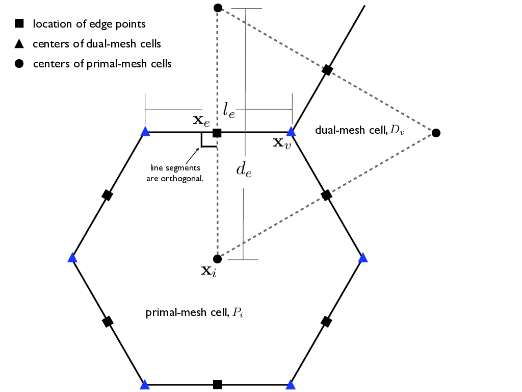
Figure C.1: Definition of elements used to build the MPAS grid. Also see Table C.1.
Table C.1
Table C.1: Definition of elements used to build the MPAS grid
Element |
Type |
Definition |
|---|---|---|
xi |
point |
location of center of primal-mesh cells |
xv |
point |
location of center of dual-mesh cells |
xe |
point |
location of edge points where velocity is defined |
de |
line segment |
distance between neighboring xi locations |
le |
line segment |
distance between neighboring xv locations |
Pi |
cell |
a cell on the primal-mesh |
Dv |
cell |
a cell on the dual-mesh |
Given a wind vector (u⊥ , u∥) defined in term of components orthogonal to and parallel to the edge, the earth-relative wind (u, v) may be recovered as
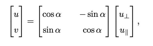
where α = angleEdge.
Table C.2
Table C:2: Variable names used to describe an MPAS grid
Element |
Name |
Size |
Comment |
|---|---|---|---|
x i |
{x,y,z}Cell |
nCells |
cartesian location of x i |
x i |
{lon,lat}Cell |
nCells |
longitude and latitude of x i |
x v |
{x,y,z}Vertex |
nVertices |
cartesian location of x v |
x v |
{lon,lat}Vertex |
nVertices |
longitude and latitude of x v |
x e |
{x,y,z}Edge |
nEdges |
cartesian location of x e |
x e |
{lon,lat}Edge |
nEdges |
longitude and latitude of x e |
d e |
dcEdge |
nEdges |
distance between x i locations |
l e |
dvEdge |
nEdges |
distance between x v locations |
e ∈ EC(i) |
edgesOnCell |
(nEdgesMax,nCells) |
edges that define P i |
e ∈ EV(v) |
edgesOnVertex |
(3,nCells) |
edges that define D v |
i ∈ CE(e) |
cellsOnEdge |
(2,nEdges) |
primal-mesh cells that share edge e |
i ∈ CV(v) |
cellsOnVertex |
(3,nVertices) |
primal-mesh cells that define D v |
v ∈ VE(e) |
verticesOnEdge |
(2,nEdges) |
dual-mesh cells that share edge e |
v ∈ VI(i) |
verticesOnCell |
(nEdgesMax,nCells) |
vertices that define P i |
Table C.3
Table C.3: Definition of element groups used to reference connections in the MPAS grid. Examples are provided in :ref:`Figure C.2`
Syntax |
Output |
|---|---|
e ∈ EC(i) |
set of edges that define the boundary of P i |
e ∈ EV(v) |
set of edges that define the boundary of D v |
i ∈ CE(e) |
two primal-mesh cells that share edge e |
i ∈ CV(v) |
set of primal-mesh cells that form the vertices of dual mesh cell D v |
v ∈ VE(e) |
the two dual-mesh cells that share edge e |
v ∈ VI(i) |
the set of dual-mesh cells that form the vertices of primal-mesh cell P i |
e ∈ ECP(e) |
edges of cell pair meeting at edge e |
e ∈ EVC(v,i) |
edge pair associated with vertex v and mesh cell i |
Figure C.2
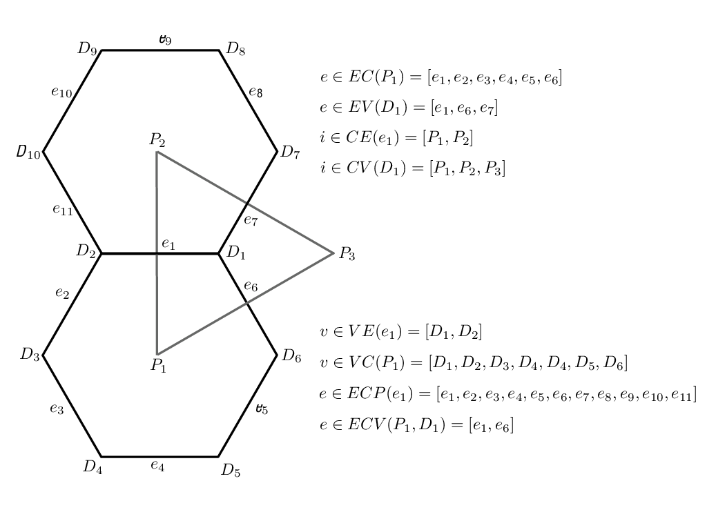
Figure C.2: Definition of element groups used to reference connections in the MPAS grid. Also see Table C.3.
Figure C.3
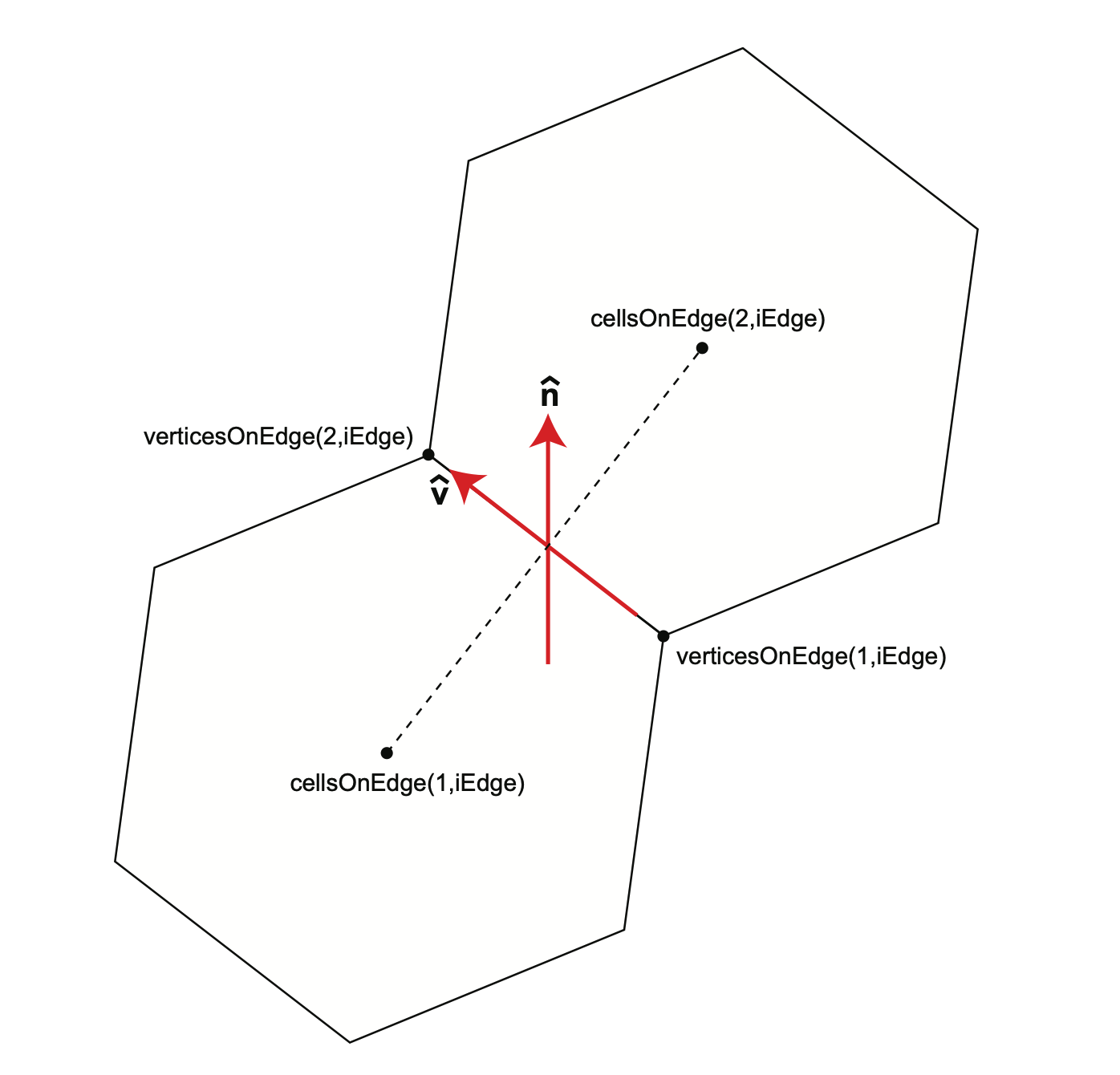
Figure C.3: The angle of an edge refers to the angle between a vector pointing north at an edge location and a vector pointing in the positive tangential velocity direction of the edge.
C.2 Vertical Grid
The vertical coordinate in MPAS-Atmosphere is ζ and has units of length, where 0 ≤ ζ ≤ zt and zt is the height of the model top. The relationship between the vertical coordinate and height in the physical domain is given as
z = ζ + Ahs ( x, y, ζ )
where (x, y) denotes a location on the horizontal mesh and ζ is the vertical coordinate (ζ is directed radially outward from the surface of the sphere, or perpendicular to the horizontal (x,y) plane in a Cartesian coordinate MPAS-A configuration). MPAS-A can be configured with the traditional Gal-Chen and Somerville terrain-following coordinate by setting hs (x, y, ζ) = h(x, y) and A = [1 - ζ / zt, where h(x, y) is the terrain height. Alternatively, A can be modified to allow a more rapid or less rapid transition to the constant-height upper boundary condition. Additionally, a constant-height coordinate can be specified at some intermediate height below ht.
The influence of the terrain on any coordinate surface ζ can be influenced by the specification of hs (x, y, ζ). Specifically, hs can be set such that hs (x, y, 0) = h(x, y) (i.e. terrain following at the sur- face), and progressively filtered fields of h(x, y) can be used at ζ>0 in hs (x, y, ζ), such that the small-scale features in the topography are quickly filtered from the coordinate. Example MPAS-A vertical meshes are given in Figure C.4.
On the MPAS-A mesh C-grid staggering, the state variables u, ρ, θ and scalars are located halfway between ω levels in both physical height and in the coordinate ζ. Variables associated with the coordinate systems used in the MPAS-A solver, and possibly appearing in its input, output or history files, are defined in Table C.4 and depicted in Figure C.5.
Further information about the vertical coordinate can be found in A Terrain-Following Coordinate with Smoothed Coordinate Surfaces.
Figure C.4
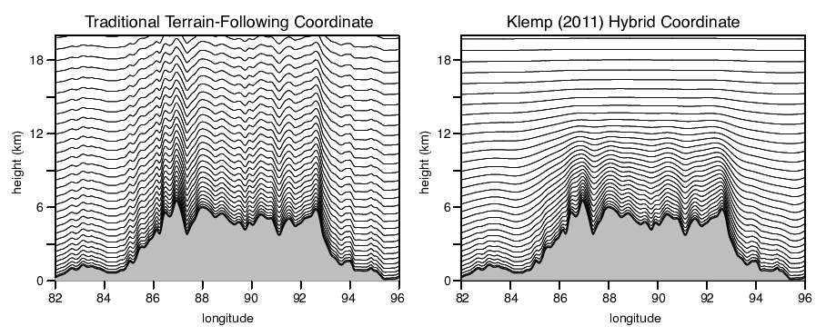
Figure C.4: Example MPAS-A vertical meshes using terrain following (left) and smoothed (right) vertical coordinates.
Table C.4
Table C.4: Vertical coordinate variables in MPAS-Atmosphere. level is the integer model level (usually specified with index k where k = 1 is the lowest model level and physical height increases with increasing k). |Delta| denotes a vertical difference between levels, and cell is a given mesh cell on the primary mesh.
Variable |
Definition |
|---|---|
zgrid(level,cell) |
physical height of the ω points in meters |
zw(level) |
ζ at ω levels |
zu(level) |
ζ at u levels; zu(k) = [z ω (k+1) + z ω (k)]/2 |
dzw(level) |
Δ ζ at u levels; dz ω (k) = z ω (k+1) - z ω (k) |
dzu(level) |
Δ ζ at ω levels; dzu(k) = [dz ω (k+1) + dz ω (k)]/2 |
rdzw(level) |
1/[dz ω ] |
rdzu(level) |
1/dzu |
zz(level,cell) |
Δ ζ / Δ z at u levels; (z ω (k+1) - z ω (k)) / (zgrid(k+1,cell) - zgrid(k,cell)) |
fzm(level) |
weight for linear interpolation to ω (k) point for u(k) level variable |
fzp(level) |
weight for linear interpolation to ω (k) point for u(k-1) level variable |
Figure C.5
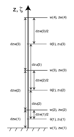
Figure C.5: Vertical distribution of the variables in MPAS-A. Also see Table C.4.