 Run with Adaptive Time Stepping Run with Adaptive Time Stepping
In this example we are going to run the same Single Domain case, but this time with Adaptive Time Stepping rather than fixed times. There is no data pre-processing necessar. As long as you still have wrfinput_d01 and wrfbdy_d01 files from a previous case, you can continue. If not, please return to the Single Domain case and generate these again.
You can read more about using Adaptive Time Stepping on page 5-23 of the ARW Users Guide.
Adaptive time stepping is a way to maximize the time step that the model can use while keeping the model numerically stable. It is typically use in for instance real-time or climate model runs to allow the model to run faster without becoming unstable.
Set-up WRF
- Make sure you are in the WRFV3 directory.
- cd to directory test/em_real
- Edit the namelist.input
file
Use the Single Domain case namelist, and add the following to the &domains section.
To ensure that the model runs fast, make sure that max_dom=1.
use_adaptive_time_step = .true.,
step_to_output_time = .true.,
target_cfl = 1.2, 1.2,
target_hcfl = .84, .84,
max_step_increase_pct = 5, 51,
starting_time_step = -1, -1,
max_time_step = 480, 480,
min_time_step = 120, 120,
adaptation_domain = 1,
Notes: Recommended min and max time steps are 4*dx and 8*dx. So we should normally start by set this to 120 and 240, but for this exercise we are just playing to see what the model will do, so we are going to set the max time high. For real-time runs or research one can make the max time step a bit higher than 8*dx, but not too high. One also needs to ensure that the min and max are not so far apart that the model time steps vary drastically. So take care when picking optimal time steps. |
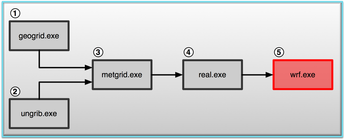
- No need to run real.exe again, just run wrf.exe:
wrf.exe
Check your output:
When running WRF with fixed time steps you would have information like this in the rsl.out.0000, showing the elapsed time for each fixed model time step:
Timing for main: time 2010-12-01_12:03:00 on domain 1: 3.43441 elapsed seconds
Timing for main: time 2006-12-19_12:06:00 on domain 1: 2.11485 elapsed seconds
Timing for main: time 2006-12-19_12:09:00 on domain 1: 2.05235 elapsed seconds
Timing for main: time 2006-12-19_12:12:00 on domain 1: 2.16914 elapsed seconds
Timing for main: time 2006-12-19_12:15:00 on domain 1: 2.05815 elapsed seconds
Timing for main: time 2006-12-19_12:18:00 on domain 1: 2.17894 elapsed seconds
Timing for main: time 2006-12-19_12:21:00 on domain 1: 2.07029 elapsed seconds
Timing for main: time 2006-12-19_12:24:00 on domain 1: 2.18028 elapsed seconds
Timing for main: time 2006-12-19_12:27:00 on domain 1: 2.09054 elapsed seconds
Timing for main: time 2006-12-19_12:30:00 on domain 1: 2.19225 elapsed seconds
When running with adaptive time step, information regarding the length of the time step will also be added to the output. You will notice that the actual time steps the model takes are also written to the log file, and that although they start lower, they quickly become longer than the original dt=180 that we used for the fixed time step runs. You might also notice that the model still outputs every 6 hours, on the hour - that is because we set step_to_output_time=.true.
Timing for main (dt=120.00): time 2006-12-20_00:02:00 on domain 1: 0.53140 elapsed seconds
Timing for main (dt=126.00): time 2006-12-20_00:04:06 on domain 1: 0.37329 elapsed seconds
Timing for main (dt=132.30): time 2006-12-20_00:06:18 on domain 1: 0.37352 elapsed seconds
Timing for main (dt=138.91): time 2006-12-20_00:08:37 on domain 1: 0.37424 elapsed seconds
Timing for main (dt=145.86): time 2006-12-20_00:11:03 on domain 1: 0.37385 elapsed seconds
Timing for main (dt=153.15): time 2006-12-20_00:13:36 on domain 1: 0.37556 elapsed seconds
Timing for main (dt=160.81): time 2006-12-20_00:16:17 on domain 1: 0.37337 elapsed seconds
Timing for main (dt=168.85): time 2006-12-20_00:19:05 on domain 1: 0.37424 elapsed seconds
Timing for main (dt=177.29): time 2006-12-20_00:22:03 on domain 1: 0.37362 elapsed seconds
Timing for main (dt=186.15): time 2006-12-20_00:25:09 on domain 1: 0.39106 elapsed seconds
Timing for main (dt=195.46): time 2006-12-20_00:28:24 on domain 1: 0.39243 elapsed seconds
Timing for main (dt=205.23): time 2006-12-20_00:31:50 on domain 1: 0.42827 elapsed seconds
Timing for main (dt=215.49): time 2006-12-20_00:35:25 on domain 1: 0.55882 elapsed seconds
Timing for main (dt=226.26): time 2006-12-20_00:39:11 on domain 1: 0.42784 elapsed seconds
Timing for main (dt=237.57): time 2006-12-20_00:43:09 on domain 1: 0.42937 elapsed seconds
Let's see the time steps the model took. Copy the
/kumquat/wrfhelp/SOURCE_CODE/WRF_NCL_scripts/wrf_AdaptiveTime.ncl script to your test/em_real directory. This script has been edited for this case, so all you need to do is get the time steps from the rsl.out.0000 file and run the script:
grep "Timing for main" rsl.out.0000 > adaptive_times.txt
ncl wrf_AdaptiveTime.ncl
This will produce the following plot on your screen.
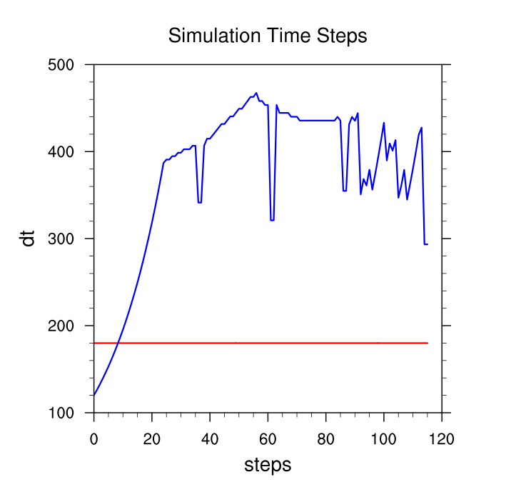
The red line represents a constant time of 180 seconds. The blue line is the actual time steps the model took. It is clear that the model mostly took time steps larger than 180 seconds. Notice the occasional big drops in time steps. This is not desirable. For this case we can see that we can set the minimum time step easily to 200 seconds, as the model take bigger time steps all the time. We want to prevent big drops in time steps and large difference in time steps, so setting the maximum time step to no more than 360 will be more sensible than our test setting of 480.
What is in the NCL script
- Reading data
To read and use the data from text files, you need to know a bit about the file you are going to read.
The data are a mix between characters and numbers and not easy to read.
So we are going to read the data with a systemfunc rather than with typical NCL read commands.
tmp = systemfunc("cut -c21-26 adaptive_times.txt")
Note that that we need to know to read characters 21-26 (so some counting is in order).
- Plotting the data
We need three pieces of information for plotting.
a. An x coordinate, which is created as a simple 0 to n array (steps)
b. A constant 180 second line, which we place in data(0,:)
c. The actual time steps the model took, which we place in data(1,:)
Note the tmp array we read is characters, and we need to convert this to floats before plotting (stringtofloat)
plot = gsn_csm_xy(wks,steps,data,res)
Organization Suggestion:
Recall the suggestion (from the "basic" case) to create a directory to put your files in. Do this again for this case:
mkdir adap_timestep
and then copy the necessary files into that directory to preserve them for potential later use.
You can now continue to run other practical examples. |