In this example we are going to generate time series output at a number of station locations. There is no data pre-processing necessary. So as long as you still have wrfinput_d01 and wrfbdy_d01 files from a previous case, you can continue. If not, please return to the Single Domain case as generate these again.

You can read more about Time Series Output on page 5-26 of the ARW Users Guide, or in WRFV3/run/README.tslist

 

 

 

Set-up WRF

• Make sure you are in the WRFV3 directory.    
   
   
• cd to directory test/em_real
   
   
• Edit the namelist.input file
  The namelist for the standard case is perfect for this example. To ensure that the model runs fast, make sure that max_dom=1.
  
  
• Create the input text file containing the station information.
  
  

Add a new text file (tslist) in the test/em_real directory. The contend of the file looks as follows: #-----------------------------------------------# # 24 characters for name | pfx  | LAT   | LON   | #-----------------------------------------------# Boulder                    kbou  40.000  -105.150 Broomfield                 kbjc  39.550  -105.070 Denver Airport             kden  39.490  -104.390 The file is format specific, so to ensure correct formatting, copy    /kumquat/wrfhelp/SOURCE_CODE/tslist to your         test/em_real directory.





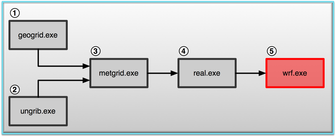
• No need to run real.exe again, just run wrf.exe:
   
             wrf.exe
   
  If successful, this will generate the following time series output files:
   
        kbou.d01.TS   kbjc.d01.TS   kden.d01.TS
        kbou.d01.PH   kbjc.d01.PH   kden.d01.PH
        kbou.d01.TH   kbjc.d01.TH   kden.d01.TH
        kbou.d01.UU   kbjc.d01.UU   kden.d01.UU
        kbou.d01.QV   kbjc.d01.QV   kden.d01.QV
        kbou.d01.VV   kbjc.d01.VV   kden.d01.VV
        
   
  pfx*.dNN.TS contains time series output of surface variables at each time step, while the others contain vertical profile data for geopotential height, potential temperature, water vapor mixing ratio, and wind at each time step.
  Note that you will have a set of text files for each pfx you specified in the tslist file.
  
   

Check your output:

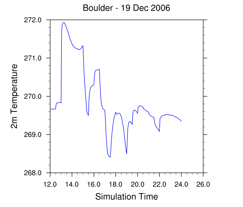
The new output files that you generated are text files, so there are any number of ways that you can look at the files or use the files. For this example we are going to plot a time series of surface temperature at the Boulder station.

Copy the /kumquat/wrfhelp/SOURCE_CODE/WRF_NCL_scripts/wrf.ts.ncl script to your test/em_real directory. This script has been edited for this case, so all you need to do is run the script  by typing

ncl wrf.ts.ncl

This will produce the following plot on your screen.

 

Now try to plot a different variable, like surface pressure. To to that you will need some explanation regarding the script

1. Reading data
   To read and use the data from text files, you need to know a bit about the file you are going to read. We know the following about this data:
      The data we are interested in are in the file kbou.d01.TS
      There are 19 columns of data in the file
       All data are real (float) values
       The file contains one header record
   Therefore we can read the data with the NCL function readAsciiTable, i.e.,
       data = readAsciiTable("kbou.d01.TS", 19, "float", 1)
   
   
2. Plotting the data
   First we need to set some plot resources to create a nice plot.
   Secondly, again we need to know something about our data before we can generate a plot.
   We know the first column in the file is a domain ID, the second is the forecast hour, and the 6th record is 2m temperature.
   If we want to plot temperature over time we will need columns 2 and 6 (this will be 1 and 5 in NCL). So we can plot the data using:
       plot = gsn_csm_xy(wks,data(:,1),data(:,5),res)
   

 

Organization Suggestion:

Recall the suggestion (from the "basic" case) to create a directory to put your files in. Do this again for this case:

mkdir time_series

and then copy the necessary files into that directory to preserve them for potential later use.

You can now continue to run other practical examples.