9. Visualization
Since the MPAS input and output files are in netCDF format, a wide variety of software tools may be used to manipulate and visualize fields in these files. As a starting point, see Plotting MPAS-A Global Simulations for access to several NCL scripts for making the basic types of plots (illustrated in Figure 1 at the end of this chapter). Each of these scripts reads the name of the file from which fields should be plotted from the environment variable FNAME, and all but the mesh-plotting script read the time frame to be plotted from the environment variable T.
To plot a field from the first frame (indexed from 0) of the file output.2010-10-23_00:00:00.nc, for example, set the following environment variables before running one of the scripts.
Note
In general, the specific field to be plotted from the netCDF file must be set within a script before running that script.
> setenv FNAME output.2010-10-23_00:00:00.nc
> setenv T 0
9.1 Meshes
To only plot an MPAS SCVT mesh, as in Figure 1(a), use the atm_mesh.ncl script. This script reads a subset of the mesh description fields from Appendix C and uses this information to draw the SCVT mesh over a color-filled map background. Parameters in the script can be used to control
the type of map projection (e.g., orthographic, cylindrical equidistant, etc.),
the colors used to fill land and water points, and
the widths of lines used for the Voronoi cells.
9.2 Horizontal Contour Plots
Horizontal field contour plots, as in Figure 1(b), can be produced with the atm_contours.ncl script. The particular field to be plotted is set in the script and can, in principle, be drawn on any horizontal surface (e.g., a constant pressure surface, a constant height surface, sea-level, etc.) if suitable vertical interpolation code is added to the script. Not shown in the figure are horizontal wind vectors, which can also be added to the plot using example code provided in the script.
9.3 Horizontal Cell-filled Plots
For visualizing horizontal fields on their native SCVT grid, the atm_cells.ncl script may be used to produce horizontal cell-filled plots, as in Figure 1(c). This script draws each MPAS grid cell as a polygon, colored according to the value of the field in that cell; the color scale is automatically chosen based on the range of the field and the default NCL color table, though other color tables can be selected instead.
9.4 Vertical Cross-sections
Vertical cross-sections of fields, as in Figure 1(d), can be created using the atm_xsec.ncl script. A starting point and ending point for the cross section must be given as latitude-longitude pairs near the top of the script, and the number of points along the cross section should be specified. The script evenly distributes the specified number of points along the shortest great-circle arc from the starting point to the ending point, and for each point, the script uses values from the grid cell containing that point (i.e., a nearest-neighbor interpolation to the horizontal cross-section points is performed); no vertical interpolation is performed, and the thicknesses and vertical heights of cells are all drawn according to the MPAS vertical grid.
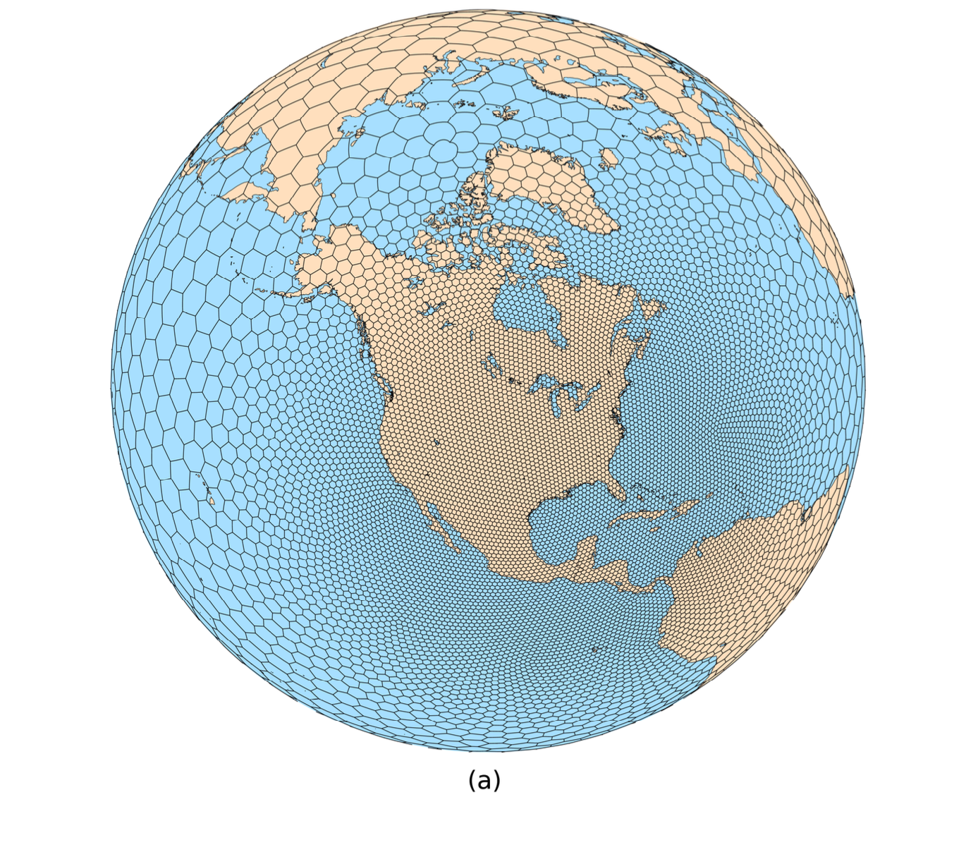
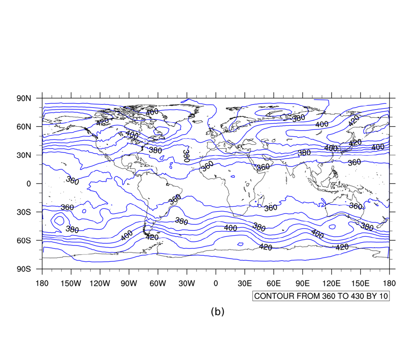
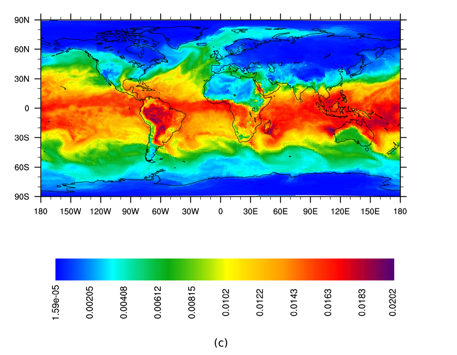
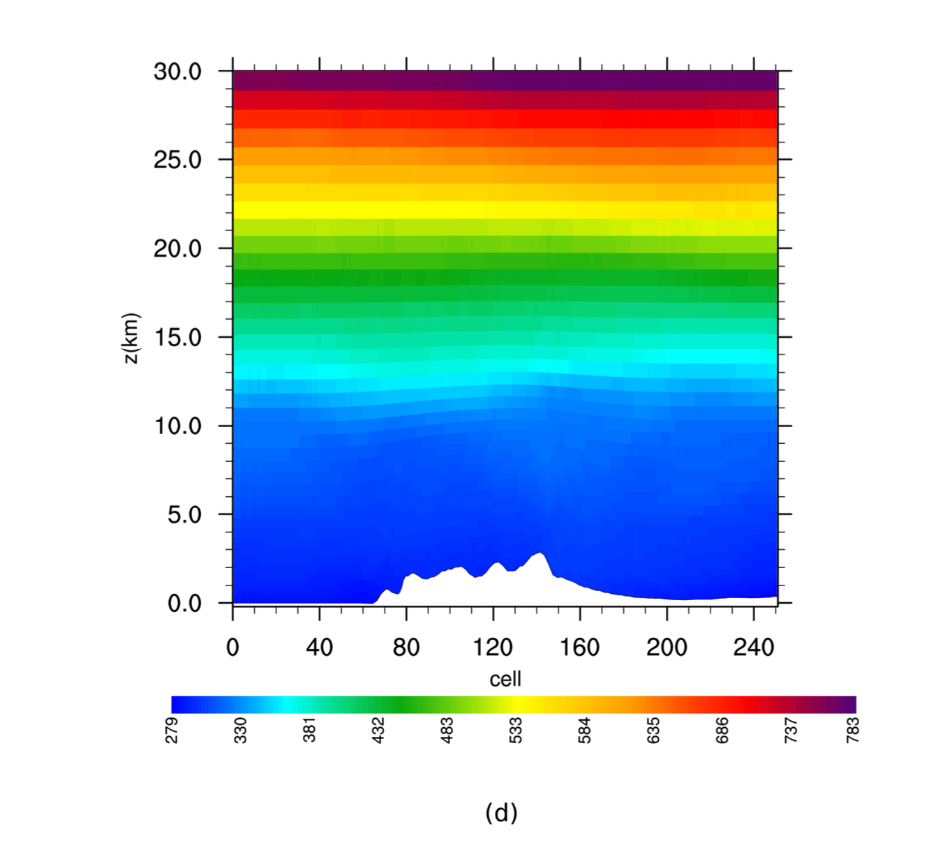
Figure 1: Various plot types that can be produced from MPAS input or output files using example scripts provided with the MPAS code. (a) A plot of an MPAS SCVT mesh against a filled map background. (b) A simple horizontal contour plot. (c) A cell-filled horizontal plot, with individual cells of the mesh drawn as polygons colored according to the field value. (d) A vertical cross-section in height, with areas below the terrain left unshaded.