Cumulus Parameterization
Physics Contents
WRF Physics Overview
Cumulus Parameterization
Microphysics
Radiation
Planetary Boundary Layer (PBL) Physics
Surface Physics
Using Physics Suites
Physics Options for Specific Applications
Cumulus Parameterization Overview
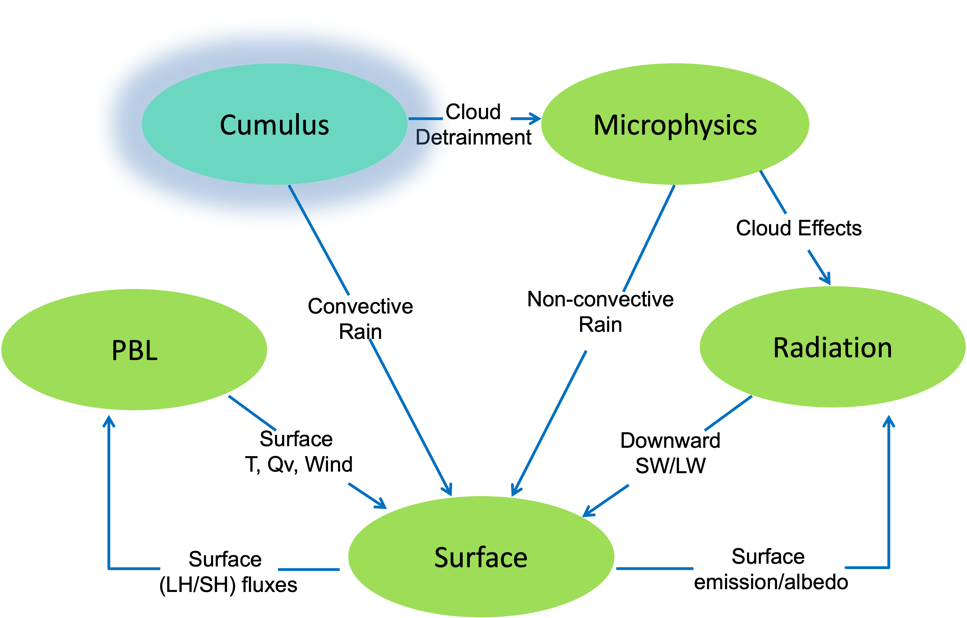

There are several cumulus schemes available and they all have varying features, but all of them parameterize sub-grid-scale effects of convective and shallow clouds. After cumulus parameterization is complete, the scheme outputs atmospheric heat and moisture tendencies to hand off to the microphysics scheme, and convective rainfall to the surface scheme.
Cumulus parameterization schemes redistribute air in gridded columns to account for vertical convective fluxes. Updrafts move boundary layer air upwards and downdrafts move mid-level air downwards. Schemes are designed to determine when to trigger a convective column and how quickly to create the convection.
All WRF cumulus schemes (except BMJ), are considered to be mass flux schemes. This means they determine updraft (and often downdraft) max flux and other fluxes, sometimes including momentum transport. Updrafts are driven by buoyancy, allowing moist surface air to rise to the upper troposphere and condensation becomes convective rainfall. Downdrafts are driven by convective rain evaporation, which cools air to the boundary layer. Subsidence warms and dries the troposphere and is the primary warming contributor in the column. The BMJ scheme is an adjustment type, and relaxes toward a post-convective (mixed) sounding.
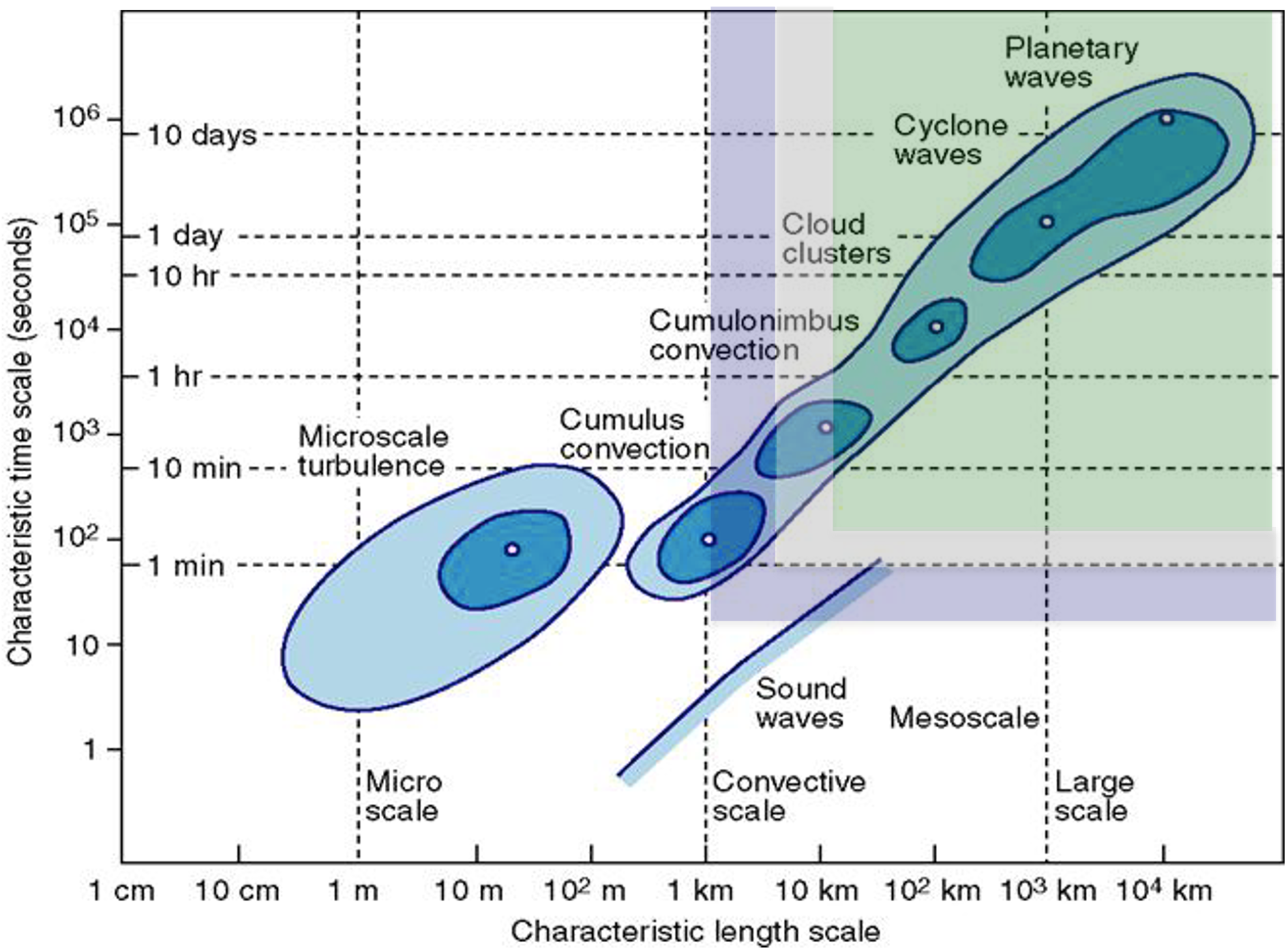
It may not always be necessary to use cumulus parameterization. It is designed for grid sizes unable to parameterize the convective processes (i.e., when updrafts and downdrafts are sub-grid).
Following are the general rules for WRF cumulus parameterization.
Domains with grid spacing >=10km : a cumulus scheme is necessary
Domains with grid spacing <=3km : unlikely that a cumulus scheme is necessary (although it may help when convection exists prior to the run)
A gray zone exists for domains with grid spacing >=3km and <=10km, and cumulus parameterization may or may not be necessary. If possible, try to avoid domains this size, but if you must use them, it is best to use either the Multi-scale Kain Fritsch or Grell-Freitas scheme, as these take this scale into account.
Note
See the `WRF Tutorial presentation on Cumulus Parameterization`_ for additional details.
Quicklinks to Cumulus Parameterization Topics
Click the following links to go directly to each topic.
Cumulus Parameterization Options
Cumulus Parameterization Option Details and References
Cumulus Parameterization Options
In the table below, moisture tendencies are mixing ratios of (c) cloud water, (r) rain water, (i) cloud ice, and (s) snow.
Scheme
Option
Moisture Tendencies
Momentum Tendencies
Shallow Convection
Radiation Interaction
Kain-Fritsch (KF)
1
Qc Qr Qi Qs
no
yes
yes
BMJ
2
N/A
no
yes
GFDL
Grell-Freitas
3
Qc Qi
no
yes
yes
Old SAS
4
Qc Qi
no
yes
GFDL
Grell-3
5
Qc Qi
no
yes
yes
Tiedtke
6
Qc Qi
yes
yes
no
Zhang-McFarlane
7
Qc Qi
yes
yes
RRTMG
KF-CuP
10
Qc Qi
no
yes
yes
Multi-scale KF
11
Qc Qr Qi Qs
no
yes
?
KIAPS SAS
14
Qc Qi
yes
use shcu_physics=4
GFDL
New Tiedtke
16
Qc Qi
yes
yes
no
Grell-Devenyi
93
Qc Qi
no
no
yes
NSAS
96
Qc Qi
yes
no/yes
GFDL
Old KF
99
Qc Qr Qi Qs
no
no
GFDL
Back to Quicklinks to Cumulus Parameterization Topics
Cumulus Parameterization Option Details and References
Kain-Fritsch (KF)
cu_physics=1
Deep and shallow convection sub-grid scheme using a mass flux approach with downdrafts and CAPE removal time scale
Kain, 2004
kfeta_trigger : =1 – default trigger; =2 – moisture-advection modulated trigger function (Ma and Tan, 2009). This option may improve results in subtropical regions when large-scale forcing is weak; =3 - RH dependent additional perturbation to option 1
cu_rad_feedback=.true. : allow sub-grid cloud fraction interaction with radiation (Alapaty et al., 2012)
Betts-Miller-Janjic (BMJ)
cu_physics=2
Operational Eta scheme. Column moist adjustment scheme relaxing towards a well-mixed profile.
Janjic, 1994Grell-Freitas (GF)
cu_physics=3
An improved GD scheme that tries to smooth the transition to cloud-resolving scales, as proposed by Arakawa et al., 2004).
Grell and Freitas, 2014Simplified Arakawa-Schubert (SAS)
cu_physics=4
Simple mass-flux scheme with quasi-equilibrium closure with shallow mixing scheme.
Pan et al., 1995Grell 3D (G3)
cu_physics=5
An improved version of the GD scheme that may also be used on high resolution (in addition to coarser resolutions) if subsidence spreading (option cugd_avedx) is turned on.
Grell, 1993
Grell and Devenyi, 2002Tiedtke scheme
cu_physics=6
(U. of Hawaii version); Mass-flux type scheme with CAPE-removal time scale, shallow component and momentum transport.
Tiedtke, 1989
Zhang et al., 2011Zhang-McFarlane
cu_physics=7
Mass-flux CAPE-removal type deep convection from CESM climate model with momentum transport.
Zhang and McFarlane, 1995Kain-Fritsch (KF) cu_physics=10
Cumulus Potential scheme; this option modifies the KF ad-hoc trigger function with one linked to boundary layer turbulence via probability density function (PDFs) using cumulus potential scheme. The scheme also computes the cumulus cloud fraction based on the time scale relevant for shallow cumuli.
Berg et al., 2013Multi-scale Kain-Fritsch
cu_physics=11
Using scale-dependent dynamic adjustment timescale, LCC-based entrainment. Also uses new trigger function based on Bechtold et al., 2001. Includes an option to use CESM aerosol. In V4.2, convective momentum transport is added. It can be turned off by setting switch cmt_opt_flag = .false. inside the code.
Zheng et al., 2016
Glotfelty et al., 2019KIAPS SAS (KSAS)
cu_physics=14
Based on NSAS, but scale-aware
Han and Pan, 2011
Kwon and Hong, 2017New Tiedtke
cu_physics=16
This version is similar to the Tiedtke scheme used in REGCM4 and ECMWF cy40r1.
Zhang and Wang, 2017Grell-Devenyi (GD)
cu_physics=93
An ensemble scheme; Multi-closure, multi-parameter, ensemble method with typically 144 sub-grid members.
Grell and Devenyi, 2002New Simplified Arakawa-Schubert (NSAS)
cu_physics=96
New mass-flux scheme with deep and shallow components and momentum transport.
Han and Pan, 2011Old Kain-Fritsch
cu_physics=99
Deep convection scheme using a mass flux approach with downdrafts and CAPE removal time scale.
Kain and Fritsch, 1990Back to Quicklinks to Cumulus Parameterization Topics
Shallow Convection
Shallow convection schemes are an additional option. Non-precipitating shallow mixing dries the planetary boundary layer, then moistens and cools above. This is done by an enhanced mixing approach or mass-flux approach. These options may be useful for grid sizes that do not resolve shallow cumulus clouds (>1 km).
Some cumulus schemes already include shallow convection:
Kain-Fritsch
Old SAS
KIAPS SAS
Grell-3
Grell-Freitas
BMJ
Tiedtke
However, to use the standalone shallow schemes, use one of the following options.
ishallow=1 : Shallow convection that works with the Grell 3D scheme (cu_physics=5)
shcu_physics=2 : UW (Bretherton and Park) Shallow cumulus option from the CESM climate model with momentum transport
Park et al., 2009shcu_physics=3 : GRIMS (Global/Regional Integrated Modeling System) scheme; represents the shallow convection process by using eddy-diffusion and the pal algorithm, and couples directly to the YSU PBL scheme
Hong and Jang, 2018shcu_physics=4 : NSAS shallow scheme; extracted from NSAS, and should be used with KSAS deep cumulus scheme
shcu_physics=5 : Deng shallow scheme; only works with MYNN and MYJ PBL schemes; (new in V4.1)
Deng et al., 2003Back to Quicklinks to Cumulus Parameterization Topics
Next section: Microphysics