Planetary Boundary Layer (PBL) Physics
Physics Contents
WRF Physics Overview
Cumulus Parameterization
Microphysics
Radiation
Planetary Boundary Layer (PBL) Physics
Surface Physics
Using Physics Suites
Physics Options for Specific Applications
Planetary Boundary Layer Overview
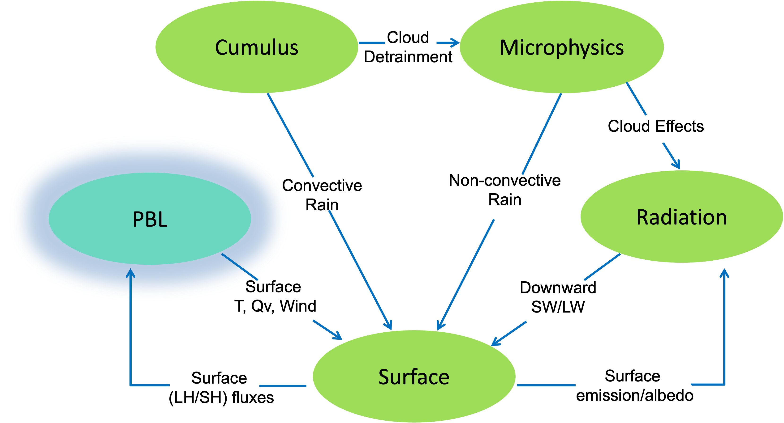

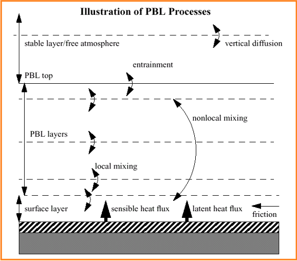
WRF Planetary Boundary Layer (PBL) schemes’ purpose is to distribute surface fluxes with boundary layer eddy fluxes, and allow for PBL growth by entrainment.
- There are two different classes of PBL schemes:
Turbulent kinetic energy prediction (Mellor-Yamada Janjic, MYNN, Bougeault-Lacarrere, TEMF, QNSE, and CAM UW). Some also include non-local mass-flux terms (QNSE-EDMF, MYNN, and TEMF)
Diagnostic non-local (YSU, GFS, MRF, ACM2)
Above the PBL, all schemes also do vertical diffusion due to turbulence.
PBL schemes can be used for most grid sizes when surface fluxes are present; however, at grid size dx << 1 km, this assumption breaks down. To get around this, you can use 3d diffusion instead of a PBL scheme (coupled to surface physics). This works best when dx and dz are comparable.
The lowest level should be in the surface layer (0.1h). This is important for surface (2m, 10m) diagnostic interpolation.
With ACM2, GFS, and MRF PBL schemes, the lowest full level should be .99 or .995 (not too close to 1).
TKE schemes and YSU can use thinner surface layers.
PBL schemes assume PBL eddies are not resolved.
Note
See the `WRF Tutorial presentation on PBL`_ for additional details.
Quicklinks to PBL Sections
Click the following links to go directly to each PBL topic.
PBL Scheme Details and References
PBL and Land Surface Time-step (bldt)
PBL Scheme Options
Scheme
Option
Works With sfclay Option
Prognostic Variables
Diagnostic Variables
Cloud Mixing
YSU
1
1 91
none
exch_h
QC QI
MYJ
2
2
TKE_PBL
EL_PBL exch_h
QC QI
QNSE-EDMF
4
TKE_PBL
EL_PBL exch_h exch_m
QC QI
MYNN2
5
1 2 5 91
QKE
Tsq Qsq Cov exch_h exch_m
QC
MYNN3
6
1 2 5 91
QKE Tsq Qsq Cov
exch_h exch_m
QC
ACM2
7
1 7 91
QC QI
BouLac
8
1 2 91
TKE_PBL
EL_PBL exch_h exch_m
QC
UW
9
1 2 91
TKE_PBL
exch_h exch_m
QC
TEMF
10
10
TE_TEMF
*_temf
QC QI
Shin-Hong
11
1 91
exch_h
QC QI
GBM
12
1 91
TKE_PBL
EL_PBL exch_h exch_m
QC QI
MRF
99
1 91
QC QI
Back to Quicklinks to PBL Sections
PBL Scheme Details and References
Yonsei University (YSU)
bl_pbl_physics=1
Non-local-K scheme with explicit entrainment layer and parabolic K profile in unstable mixed layer; includes capability of topdown mixing for turbulence driven by cloud-top radiative cooling, which is separate from bottom-up surface-flux-driven mixing
Hong et al., 2006Additional options specific for use with YSU:
topo_wind : =1 - topographic correction for surface winds to represent extra drag from sub-grid topography and enhanced flow at hill tops (Jimenez and Dudhia, 2012); =2 - a simpler terrain variance-related correction
ysu_topdown_pblmix=1 : option for top-down mixing driven by radiative cooling
Mellor-Yamada-Janjic (MYJ)
bl_pbl_physics=2
Eta operational scheme; one-dimensional prognostic turbulent kinetic energy scheme with local vertical mixing
Janjic, 1994
Mesinger, 1993Quasi-Normal Scale Elimination (QNSE-EDMF)
bl_pbl_physics=4
A TKE-prediction option that uses a new theory for stably-stratified regions; daytime part uses eddy diffusivity mass-flux method with shallow convection (mfshconv = 1); includes shallow convection using a mass-flux approach through the whole cloud-topped boundary layer
Sukoriansky et al., 2005Mellor-Yamada Nakanishi and Niino Level 2.5 (MYNN2)
bl_pbl_physics=5
Predicts sub-grid TKE terms; includes shallow convection using a mass-flux approach through the whole cloud-topped boundary layer; includes a capability of top-down mixing for turbulence driven by cloud-top radiative cooling, which is separate from bottom-up surface-flux-driven mixing
Nakanishi and Niino, 2006
Nakanishi and Niino, 2009
Olson et al., 2019Additional options specific for use with MYNN:
icloud_bl=1 : option to couple subgrid-scale clouds from MYNN to radiation
bl_mynn_cloudpdf : =1 - Kuwano et al., 2010 ; =2 - Chaboureau and Bechtold, 2002 (with mods, default)
bl_mynn_cloudmix=1 : mixing cloud water and ice (qnc and qni are mixed when scalar_pblmix=1)
bl_mynn_edmf=1 : activate mass-flux in MYNN
bl_mynn_mixlength : =1 is from RAP/HRRR; =2 is from blending
Mellor-Yamada Nakanishi and Niino Level 3 (MYNN3)
bl_pbl_physics=6
Predicts TKE and other second-moment terms
Nakanishi and Niino, 2006
Nakanishi and Niino, 2009
Olson et al., 2019ACM2
bl_pbl_physics=7
Asymmetric Convective Model with non-local upward mixing and local downward mixing
Pleim, 2007BouLac
bl_pbl_physics=8
Bougeault-Lacarrère PBL; a TKE-prediction option; designed for use with BEP urban model
Bougeault, 1989UW
bl_pbl_physics=9
TKE scheme from CESM climate model; includes shallow convection using a mass-flux approach from the cloud base; includes capability of topdown mixing for turbulence driven by cloud-top radiative cooling, which is separate from bottom-up surface-flux-driven mixing
Bretherton and Park, 2009Total Energy - Mass Flux (TEMF)
bl_pbl_physics=10
Sub-grid total energy prognostic variable, plus mass-flux type shallow convection; includes shallow convection using a mass-flux approach through the whole cloud-topped boundary layer
Angevine et al., 2010Shin-Hong
bl_pbl_physics=11
Includes scale dependency for vertical transport in convective PBL; vertical mixing in the stable PBL and free atmosphere follows YSU; this scheme also has diagnosed TKE and mixing length output
Shin and Hong, 2015Grenier-Bretherton-McCaa (GBM)
bl_pbl_physics=12
A TKE scheme; tested in cloud-topped PBL cases; includes shallow convection using a mass-flux approach from the cloud base
Grenier and Bretherton, 2001TKE (E)-TKE dissipation rate (epsilon) (EEPS)
bl_pbl_physics=16
This scheme predicts TKE, as well as TKE dissipation rate; it also advects both TKE and the dissipation rate; Only works with sf_sfclay_physics options 1, 91, and 5
No publication availableMRF
bl_pbl_physics=99
Older version of YSU (option 1) with implicit treatment of entrainment layer as part of non-local-K mixed layer
Hong and Pan, 1996Back to Quicklinks to PBL Sections
Additional PBL Options
LES PBL
Settings for a large-eddy-simulation (LES) boundary layer:bl_pbl_physic = 0
isfflx = 1
sf_sfclay_physics = any option, except 0
sf_surface_physics = any option, except 0
diff_opt = 2
km_opt = 2 or 3This uses diffusion for vertical mixing. Alternative idealized ways of running the LES PBL are chosen with “isfflx = 0 or 2”. It is best to use dx~dz, especially in the boundary layer, and avoid stretching to very large dz/dx aspect ratios at upper levels. This also tends to work better with continuous stretching to the top, rather than with fixed upper-level dz when dz >> dx.
SMS-3DTKE
This is a 3D TKE subgrid mixing scheme that is self-adaptive to the grid size between the large-eddy simulation (LES) and mesoscale limits (new since V4.2). It can be activated by settingbl_pbl_physic = 0
km_opt = 5
diff_opt = 2
sf_sfclay_physics = 1, 5, or 91Gravity Wave Drag
gwd_opt
Can be used for all grid sizes with appropriate input fields from geogrid to represent sub-grid orographic gravity-wave vertical momentum transport
=1 : (default); gravity wave drag and blocking; recommended for all grid sizes; includes the subgrid topography effects gravity wave drag and low-level flow blocking; input wind is rotated to the earth coordinate, and output is adjusted back to the projection domain - this enables the scheme to be used for all map projections supported by WRF; to apply this option, appropriate input fields from geogrid must be used; see the (kkw - link) Selecting Static Data for the Gravity Wave Drag Scheme in Chapter 3 of this guide for details
=3 : gravity wave drag, blocking, small-scale gravity drag and turbulent orographic form drag; similar to option 1, with an additional two subgrid-scale sources of orographic drag: one is small-scale GWD (Tsiringakis et al., 2017), which represents gravity wave propagation and breaking in and above stable boundary layers; the other is the turbulent orographic form drag of Beljaars et al., 2004. Both are applicable down to a grid size of 1 km. Large-scale GWD and low-level flow blocking from gwd_opt=1 are properly adjusted for the horizontal grid resolution. More diagnostic fields from the scheme can be output by setting namelist option “gwd_diags=1.” New GWD input fields are required from WPS.
Fog
grav_settling=2
Gravitational settling of fog/cloud dropletsBack to Quicklinks to PBL Sections
PBL and Land Surface Time-step (bldt)
“bldt” is a namelist.input parameter used to determine the minutes between boundary layer and land-surface model calls. The typical value is 0 (every step), and this is reasonable for all schemes, with the exception of the CSM land-surface scheme. CSM LSM is expensive, so it may be better to consider increasing the value of bldt when using it.
Back to Quicklinks to PBL Sections
Model Grid Spacing
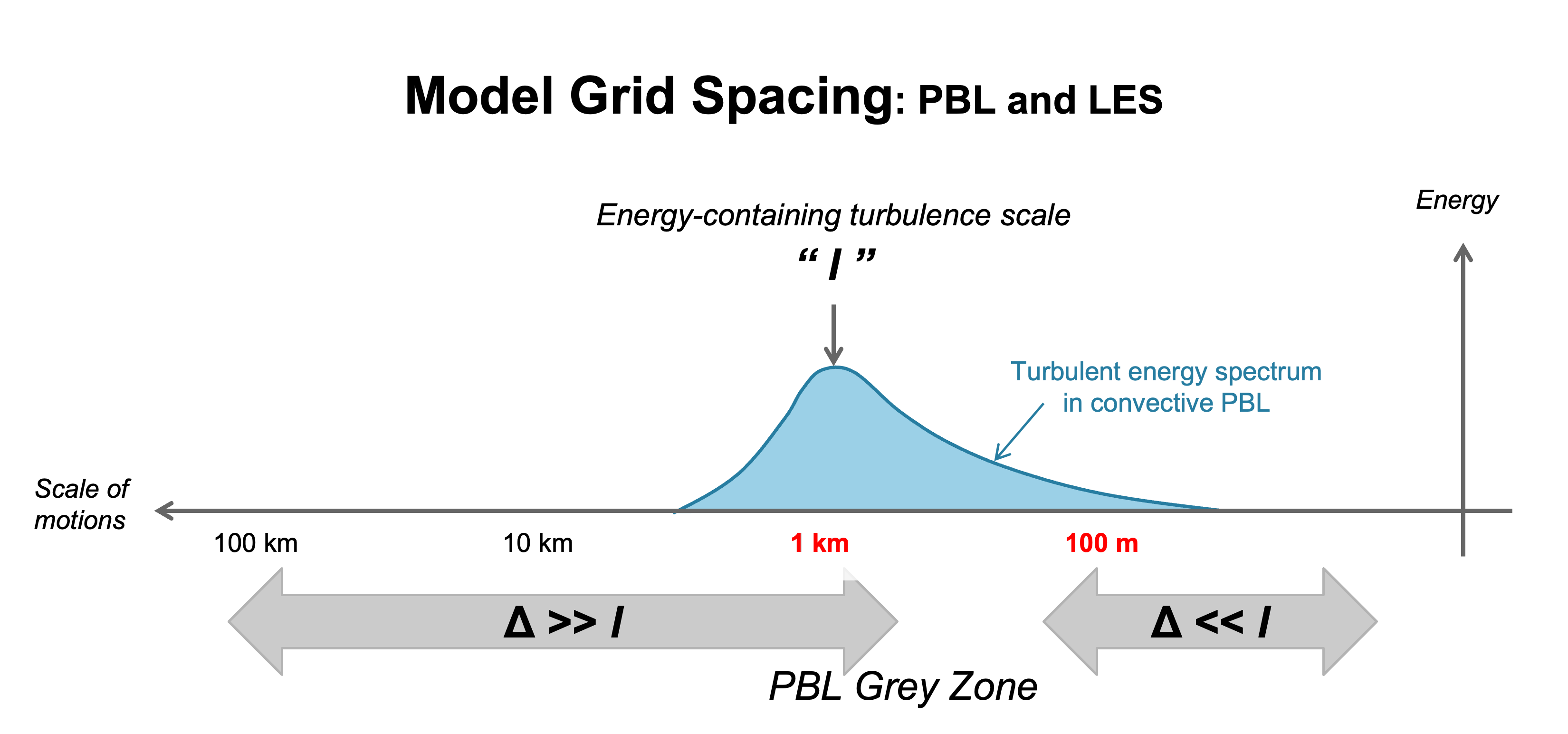
WRF PBL schemes are designed for grid resolution >> I in the image above, while LES schemes are designed for grid resolution << I. For coarse grid spacing, all eddies are sub-grid, and 1-D column schemes handle sub-grid vertical fluxes. For fine grid spacing, all major eddies are resolved, and 3-D turbulence schemes handle sub-grid mixing.
The remaining grid-spacing is a grey-zone, which is sub-kilometer grids, where PBL and LES assumptions are not perfect. There are scale-aware schemes that can be used for this zone.
Shin-Hong PBL based on YSU, designed for sub-kilometer transition scales (200 m – 1 km); nonlocal mass-flux and Kv term is reduce in strength as the grid size gets smaller and resolved mixing increases
New 3d TKE option (km_opt=5) in V4.2; becomes 3-D LES at fine scales; adds scale-dependent Shin-Hong nonlocal mass flux and implicit vertical diffusion at coarse grid sizes
Other schemes may work in this range but will not have correctly partitioned resolved/sub-grid energy fractions
For grid sizes up to about 100m, LES is preferable.
Back to Quicklinks to PBL Sections
Turbulence and Diffusion
The namelist.input parameter “diff_opt” is used to specify the turbulence and mixing option. When diffusion is used with a PBL scheme, vertical diffusion is deactivated, so diff_opt only affects horizontal diffusion.
diff_opt=0 : no turbulence or explicit spatial numerical filters
diff_opt=1 : (default); evaluates the 2nd-order diffusion term on coordinate surfaces; limited to constant vertical diffusion coefficient (kvdif); should not be used with calculated diffusion coefficient options (km_opt=2,3); can be used with PBL schemes that include vertical diffusion internally; horizontal diffusion acts along model levels; simple numerical method with only neighboring points on the same model level
diff_opt=2 : evaluates mixing terms in physical space (stress form - x,y,z); strictly horizontal and better for complex terrain - avoids diffusion up and down slopes included in “diff_opt=1;” horizontal diffusion acts on strictly horizontal gradients; numerical method includes vertical correction term, using more grid points; for stability, diffusion strength is reduced in steep coordinate slopes (dz ~ dx)
Recommended Diffusion Options
- Real-data case with PBL option on
diff_opt=2
km_opt=4
Less diffusive in complex terrain (while diff_opt=1 diffuses along slopes)
These options compliment vertical diffusion done by the PBL scheme
- High-resolution real-data cases (~100m grid)
No PBL scheme
diff_opt=2
km_opt=2 or 3 (TKE or Smagorinsky scheme)
- Idealized cloud-resolving (dx= 1-3 km) modeling (smooth or no topography, no surface heat fluxes)
diff_opt=2
km_opt=2 or 3
- Complex topography with no PBL scheme
diff_opt=2 is more accurate for sloped coordinate surfaces, and prevents diffusion up/down valley sides, but can still potentially be unstable with complex terrain
WRF is incapable of handling slopes > 45 degrees - can use “epssm,” which is a damping term that can be increased to help with steep slopes (e.g., 0.5-1.0)
Back to Quicklinks to PBL Sections
Next section: Surface Physics