Meshes & Mesh Utilities
Several resolutions of quasi-uniform and refined meshes are available for download. Each mesh download provides the following:
an SCVT mesh on the unit sphere
the mesh connectivity (graph.info) file for the mesh
partitionings of the mesh (e.g., graph.info.part.32) for various MPI task counts
Additionally, for quasi-uniform meshes, “static” files using the default datasets are available. The static file downloads provide single-precision static files in CDF-5/64-bit data format and mesh connectivity files.
Creating limited-area subsets of meshes
MPAS-Atmosphere includes the capability to perform regional simulations. Regional meshes are formed as subsets of existing meshes. The MPAS-Limited-Area Python tool is the supported method for generating regional meshes as subsets of any of the meshes or static files available from the “Download” links below. Please refer to the documentation provided with MPAS-Limited-Area for details of its use.
Projecting Perfect Hexagonal Meshes onto the Sphere Using Standard Projections
This utility provides the capability of creating a regional MPAS horizontal mesh by projecting a rectangular mesh composed of perfect hexagons to the sphere using a Lambert conformal projection. The utility is found in the MPAS-Tools Github repository and it can be found in MPAS-Tools/mesh_tools/hex_projection. The README file provides directions for building and running the utility.
Scaling Regional Meshes
The scale_region.py tool is used to scale the sizes of elements in a regional MPAS mesh, so that the resulting Voronoi cells and Delaunay triangles are some factor of their original size. Typically, a coarser regional mesh is scaled to higher resolution, with a corresponding decrease in the area covered by the mesh.
Quasi-uniform Meshes and Static Fields
Click on links in the “File” column below to download the mesh and static file needed.
Resolution |
# of horizontal grid cells |
File |
|---|---|---|
480 km |
2562 |
480-km mesh (1.5 MB) |
384 km |
4002 |
384-km mesh (2.4 MB) |
240 km |
10242 |
240-km mesh (6.3 MB) |
120 km |
40962 |
120-km mesh (25.7 MB) |
60 km |
163842 |
60-km mesh (106 MB) |
48 km |
256002 |
48-km mesh (182 MB) |
30 km |
655362 |
30-km mesh (436 MB) |
24 km |
1024002 |
24-km mesh (685 MB) |
15 km |
2621442 |
15-km mesh (1659 MB) |
Dense Meshes
Note
The 3-d fields that exist in the model at higher resolution can easily exceed the 4 GB limit imposed by the classic netCDF format. When creating atmospheric initial conditions (i.e., the “init.nc” file), and when writing output streams from the model with 3-d fields, it is necessary to use an “io_type” that supports large variables, such as “pnetcdf,cdf5” or “netcdf4”. For more information on selecting the “io_type” of a stream, refer to Configuring Model Input and Output from the MPAS-A Users’ Guide.
Note that when processing GWDO static fields, each MPI task needs to allocate ~4 GB of additional memory to hold the global 30-arc-second terrain dataset. In many cases it may be necessary to under-subscribe batch nodes to avoid exceeding memory limits.
Resolution |
# of horizontal grid cells |
File |
|---|---|---|
12 km |
4096002 |
12-km mesh (2713 MB) |
10 km |
5898242 |
10-km mesh (3916 MB) |
7.5 km |
10485762 |
7.5-km mesh (6936 MB) |
5 km |
23592962 |
5-km mesh (15487 MB) |
4 km |
36864002 |
4-km mesh (23721 MB) |
3.75 km |
41943042 |
3.75-km mesh (27246 MB) |
3 km |
65536002 |
3-km mesh (42007 MB) |
Variable-resolution Meshes
All variable-resolution meshes are supplied with a single refinement region that is centered on 0.0 degree latitude, 0.0 degree longitude. This region of refinement may be relocated to other locations on the sphere using the “grid_rotate”, whose usage is described in Preparing Meshes from the MPAS-A Users’ Guide.
92-25 km Mesh
This mesh contains 163,842 horizontal grid cells, with the refinement region spanning approximately 60 degrees of latitude/longitude.
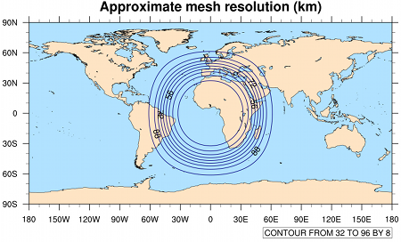
Download the 92-25 km mesh (135 MB)
46-12 km Mesh
This mesh is like the 92-km to 25-km mesh, but with twice the horizontal resolution and 655,362 horizontal grid cells.
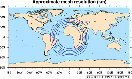
Download the 46-12 km mesh (592 MB)
60-15 km Mesh
This mesh contains 535,554 horizontal grid cells, with the refinement region spanning approximately 55 degrees of latitude and 110 degrees of longitude.
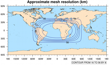
Download the 60-15 km mesh (474 MB)
60-10 km Mesh
This mesh contains 999,426 horizontal grid cells, with the refinement region spanning approximately 80 degrees of latitude/longitude.
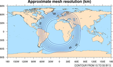
Download the 60-10 km mesh (913 MB)
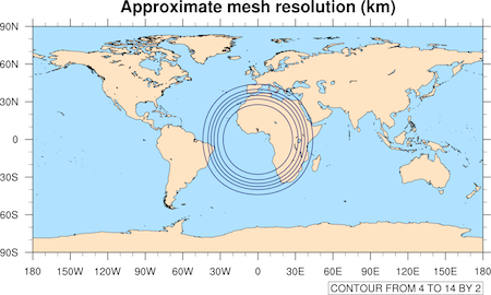
60-3 km Mesh
This mesh contains 835,586 horizontal grid cells, with the refinement region spanning approximately 16 degrees of latitude/longitude.
Download the 60-3 km mesh (628 MB)
60-15 km (Tropical Refinement) Mesh
This mesh contains 1,572,866 horizontal grid cells, with the refinement region spanning the tropics.
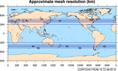
Download the 60-15 km (Tropical Refinement) mesh (1177 MB)
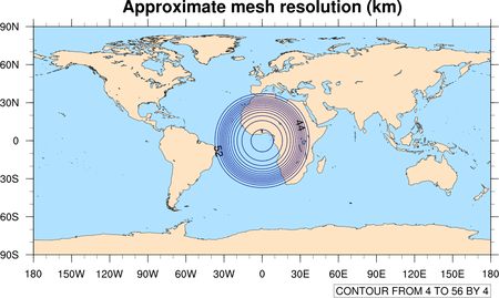
15-3 km (Circular Refinement) Mesh
This mesh contains 6,488,066 horizontal grid cells, with the circular refinement region spanning approximately 60 degrees of latitude/longitude. When using this mesh, the following steps are required.
The 3-d fields that exist in the model at higher resolution can exceed the 4 GB limit imposed by the classic netCDF format. When creating atmospheric initial conditions (i.e., the “init.nc” file), and when writing output streams from the model with 3-d fields, it is necessary to use an “io_type” that supports large variables, such as “pnetcdf,cdf5” or “netcdf4”. For more information on selecting the “io_type” of a stream, refer to Configuring Model Input and Output from the MPAS-A Users’ Guide.
When processing GWDO static fields, each MPI task needs to allocate ~4 GB of additional memory to hold the global 30-arc-second terrain dataset. In many cases, it may be necessary to under-subscribe batch nodes to avoid exceeding memory limits.
When running the model with the 15-km to 3-km mesh, set config_apvm_upwinding=0.0 in the nhyd_model namelist record.
Download the 15-3 km (Circular Refinement) mesh (4560 MB)
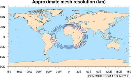
15-3 km (Elliptical Refinement) Mesh
This mesh contains x5.8060930 horizontal grid cells, with the elliptical refinement region spanning approximately 60 degrees of latitude and 80 degrees of longitude. When using this mesh, the following changes are required.
The 3-d fields that exist in the model at higher resolution can exceed the 4 GB limit imposed by the classic netCDF format. When creating atmospheric initial conditions (i.e., the “init.nc” file), and when writing output streams from the model with 3-d fields, it is necessary to use an “io_type” that supports large variables, such as “pnetcdf,cdf5” or “netcdf4”. For more information on selecting the “io_type” of a stream, refer to Configuring Model Input and Output from the MPAS-A Users’ Guide.
When processing GWDO static fields, each MPI task needs to allocate ~4 GB of additional memory to hold the global 30-arc-second terrain dataset. In many cases, it may be necessary to under-subscre batch nodes to avoid exceeding memory limits.
When running the model with the 15-km to 3-km mesh, set config_apvm_upwinding=0.0 in the nhyd_model namelist record.
Download the 15-3 km (Elliptical Refinement) mesh (5963 MB)