Running WRF

By default, the WRF model is a fully compressible, nonhydrostatic model with a hybrid vertical hydrostatic pressure coordinate (HVC), and Arakawa C-grid staggering. The model uses the Runge-Kutta 2nd and 3rd order time integration schemes, and 2nd to 6th order advection schemes in both the horizontal and vertical. It uses a time-split small step for acoustic and gravity-wave modes. The dynamics conserve scalar variables.

WRF model code contains the following programs:

real.exe or ideal.exe

An initialization program for either real-data (real.exe) or idealized data (ideal.exe)

wrf.exe

A numerical integration program

ndown.exe

A program allowing one-way nesting for domains run separately

tc.exe

A program for tropical storm bogussing

Version 4 of the WRF model supports a variety of capabilities, including

• Real-data and idealized simulations

• Various lateral boundary condition options

• Full physics options, with various filters

• Positive-definite advection scheme

• Hydrostatic runtime option

• Terrain-following vertical coordinate option

• One-way, two-way, and moving nest options

• Three-dimensional analysis nudging

• Observation nudging

• Regional and global applications

• Digital filter initialization

• Vertical refinement for a nested domain

Running Idealized Cases

An idealized simulation may be run once the WRF model is successfully compiled for one of the idealized test cases. The following two executables are built with the code and should be available in the WRF/main directory, and linked from there to the WRF/test/em_case directory, where case refers to the specific idealized simulation (see Available Ideal Test Cases).

• ideal.exe

  The Idealized Case Initialization program for the test case

• wrf.exe

  The primary numerical integration program

Steps to Run an Idealized Simulation

The following instructions are specific to the “3-D Baroclinic Wave Case,” but the directions may generally be applied when running other idealized cases, as well (making modifications where necessary). All commands are issued in a terminal window environment.

1. Move to the test case directory.

   cd WRF/test/em_b_wave
   

   
   

2. Edit the namelist.input file to set integration length, output frequency, domain size, timestep, physics options, and other parameters (see README.namelist in the WRF/run directory, or Namelist Variables), and then save the file.

   
   

3. Run the ideal initialization program.

   
   

   For a “serial” code build:

   ./ideal.exe >& ideal.log
   

   
   

   For code built for parallel computing (e.g., dmpar):

   mpirun -np 1 ./ideal.exe
   

   
   

   Note

   ideal.exe must be run with only a single processor (denoted by “-np 1”), even if the code is built for parallel computing. Later, wrf.exe may be run with multiple processors.

   
   

   ideal.exe typically reads an input sounding file provided in the case directory, and generates an initial condition file, wrfinput_d01. Idealized cases do not require a lateral boundary file because boundary conditions are handled in the code via namelist options. If the job is successful, the phrase SUCCESS COMPLETE IDEAL INIT should be present at the end of the ideal.log (or rsl.out.0000 for parallel execution).

   
   

4. Run the WRF model.

   
   

   For a “serial” code build:

   ./wrf.exe >& wrf.log
   

   
   

   For code built for parallel computing (where here 8 processors are requested):

   mpirun -np 8 ./wrf.exe
   

When the run is complete, a successful simulation will print SUCCESS COMPLETE WRF at the end of the wrf.log file (or rsl.out.0000 for parallel execution). The following new files may be present, depending on user settings:

• rsl.out.* and rsl.error.*

  (For MPI runs only) Pairs of WRF model standard out and error files, one each for each processor used

• wrfout_d0x_YYYY-MM-DD_hh:mm:ss

  The WRF model output, where x denotes the domain ID, and the remaining variables represent the date and time for which the file is valid

• wrfrst_d0x_YYYY-MM-DD_hh:mm:ss

  Files that may be used to restart a simulation. They are created if the restart_interval setting in the namelist.input file is within the total simulation time. Here, x denotes the domain ID, and the remaining variables represent the date and time for which the file is valid.

See Idealized Case Initialization for additional information on idealized cases, including code modification and backward compatibility for idealized cases.

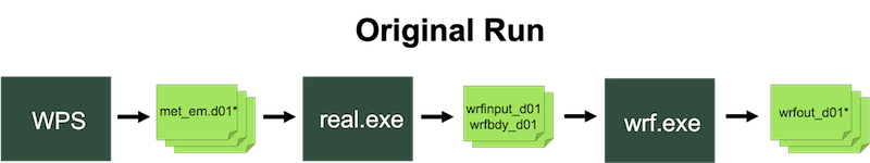
Running Real-data Cases

1. To run the model for a real-data case, move to the working directory by issuing the command

   cd WRF/test/em_real
   

   
   

   Note

   Real data cases can also be run in the WRF/run directory.

   
   

2. Prior to running a real-data case, the WRF Preprocessing System (WPS) must have been successfully run, producing met_em.* output files that will be used as input to the real.exe program. Link the met_em* files to the WRF running directory.

   ln -sf ../../../WPS/met_em* .
   

   
   

3. Start with the default namelist.input file available in the running directory and edit it for your case.

   • Set the parameters in the &time_control and &domains records specific to your case.

   • Set dates and domain dimensions to match those set in WPS. If only one domain is used, only entries in the first column are read and other columns are ignored. No need to remove additional columns.

   
   

4. Run the real-data initialization program by issuing the following commands, based on the type of compile used.

   
   

   For WRF built for serial computing, or OpenMP (smpar)

   ./real.exe >& real.log
   

   
   

   For WRF built for parallel computing (dmpar) - an example requesting to run with four processors

   mpiexec -np 4 ./real.exe
   

   
   

   If successful, the end of real.log (or rsl.out.0000 file for dmpar simulation) should read real_em: SUCCESS EM_REAL INIT and wrfinput_d0* files (one file per domain) and a wrfbdy_d01 file should be available in the running directory. These files are used as input to the wrf.exe program.

   
   

5. Run the WRF model.

   
   

   For WRF built for serial computing, or OpenM (smpar)

   ./wrf.exe >& real.log
   

   
   

   For WRF built for parallel computing (dmpar) - an example requesting to run with four processors

   mpiexec -np 4 ./wrf.exe
   

   
   

When the run is complete, a successful simulation will print SUCCESS COMPLETE WRF at the end of the wrf.log file (or rsl.out.0000 for parallel execution). The following new files may be present, depending on user settings:

• rsl.out.* and rsl.error.*

  (For MPI runs only) Pairs of WRF model standard out and error files, one each for each processor used

• wrfout_d0x_YYYY-MM-DD_hh:mm:ss

  The WRF model output, where x denotes the domain ID, and the remaining variables represent the date and time for which the file is valid; multiple wrfout files may exist, and/or multiple time periods may be included in each file, depending on the user settings for namelist options history_interval and

• wrfrst_d0x_YYYY-MM-DD_hh:mm:ss

  Files that may be used to restart a simulation. They are created if the restart_interval setting in the namelist.input file is within the total simulation time. Here, x denotes the domain ID, and the remaining variables represent the date and time for which the file is valid.

Check the times written to any netCDF output file by issuing something similar to the following (specify the actual name of a single file):

ncdump -v Times wrfout_d0x_YYYY-MM-DD_hh:mm:ss

Restart Capability

The restart option extends a run to a longer simulation period when there is a reason it cannot be simulated in a single run (for e.g., the run extends beyond available wallclock time for queueing systems). It is a continuous run made of two ore more shorter runs. The results at the end of one or more restart runs should be identical to a single run without a restart, though there may be specific options known to not produce bit-for-bit results (see WRF Known Problems & Solutions).

To initiate the restart:

1. Prior to the initial simulation set restart_interval in the namelist.input to a value (in minutes) equal to or less than the initial simulation’s length. This instructs wrf.exe to write out a restart file when the model reaches the restart_interval. Restart files use the naming convention wrfrst_d<domain>_<date>, where the date string represents the time when the restart file is valid.

   
   

2. After the initial simulation completes, and there is a valid wrfrst_d<domain>_<date> file available, modify the namelist again by setting:

   • start_time = the restart time (<date> of the restart file; in &time_control)

   • restart = .true. (in &time_control)

3. Run wrf.exe as usual.

The following additional namelist options are available to use for restarts:

• override_restart_timers=.true.

  Use this if the history and/or restart interval are modified prior to the restart run, and the new output times are not as expected (in &time_control)

• write_hist_at_0h_rst=.true.

  If history output is desired at the initial time of the restart simulation (in &time_control)

Note

Restart files are typically several times the size of history files. The model may be capable of writing history files (wrfout files) in netCDF format, but may fail to write a restart file due to the large file size. If this is the case, try setting io_form_restart=102 (instead of 2), which forces the restart file to be written into multiple pieces, one per processor. As long as the model is restarted using the same number of processors (which is the recommended practice anyway), this option works well.

WRF Nesting

Nested Simulation

A simulation in which a coarse-resolution domain (parent) contains at least one embedded finer-resolution domain (child)

Nested domains can be run together simultaneously, or separately. The nest receives data driven along its lateral boundaries from its parent, and depending on the namelist setting for feedback, the nest may also provide data back to the parent.

See the WPS section on Nested Domains to determine whether to use a nest.

The below sections discuss the following different available nesting options:

• Basic Nesting

• One-way Nesting Using Ndown

• Automatic Moving Nests (Vortex-following)

• Specified Moving Nests

Basic Nesting

Simulating WRF with basic nesting includes multiple domains at different grid resolutions that are run simultaneously and communicate with each other using either one-way or two-way nesting, determined by the namelist.input setting for feedback.

Two-way Nesting

feedback=1
The coarser (parent) domain provides boundary data for the higher-resolution nest (child), and the nest feeds its calculations back to the coarser domain. The model can handle multiple domains at the same nest level (no overlapping nests), and multiple nest levels (telescoping).

One-way Nesting

feedback=2
Communication only goes in one direction - from the parent domain to the child domain. There is no feedback to the parent.

When preparing for a nested run, make sure code is compiled with “basic” nest option (option 1).

Nesting options are declared in the namelist. Variables that have multiple columns need to be edited (to avoid errors, do not add columns to namelist parameters that do not have multiple column values in the default namelist). Start with the default namelist. The following are the key namelist variables to modify:

Note

See Namelist Variables for additional descriptions of the following list of variables.

feedback	this determines whether the simulation is a two-way or one-way nested run. feedback=1 turns on feedback; values of the coarse domain are overwritten by values of the variables (average of cell values for mass points, and average of the cell-face values for horizontal momentum points) in the nest at coincident points; for masked fields, only the single point value at the collocating points is fed back; if parent_grid_ratio is even, an arbitrary choice of the southwest corner point value is used for feedback, which is why it is better to use an odd parent_grid_ratio when feedback=1 feedback=0 turns feedback off; it is equivalent to a one-way nested run, since nest results are not reflected in the parent domain
start_* end_*	start and end simulation times for all domains
input_from_file	set to .true. or .false., indicating whether a nest requires an input file (e.g. wrfinput_d02). This is typically used for real data cases since the nest input file contains nest topography and land information.
fine_input_stream	determines which fields (defined in Registry/Registry.EM_COMMON) from the nest input file are used in nest initialization. This typically includes static fields (e.g., terrain and landuse), and masked surface fields (e.g., skin temperature, soil moisture and temperature). This option is useful for a nest starting at a later time than the coarse domain.
max_dom	the total number of domains to run. For e.g., for one coarse domain and one nest, set max_dom=2.
grid_id	domain identifier used in the wrfout naming convention. The most coarse grid must have a grid_id of 1.
parent_id	indicates each nests’s parent domain. This should be set as the grid_id value of the parent (e.g., d02’s parent is d01, so parent_id for column two should be set to 1).
i_parent_start j_parent_start	lower-left corner starting indices of the nest domain within its parent domain. These parameters should be the same as in namelist.wps.
parent_grid_ratio	integer grid size (resolution) ratio of the child domain to its parent. Typically odd number ratios are used in real-data applications (ratios of 3:1 and 5:1 have shown the best results; it is not recommended to use a ratio larger than 5:1).
parent_time_step_ratio	integer time-step ratio for the nest domain, which can be different from the parent_grid_ratio, though they are typically set the same.
smooth_option	a smoothing option for the parent domain in the area of the nest if feedback is on. Three options are available: 0 = no smoothing; 1 = 1-2-1 smoothing; 2 = smoothing-desmoothing.

One-way Nesting Using Ndown

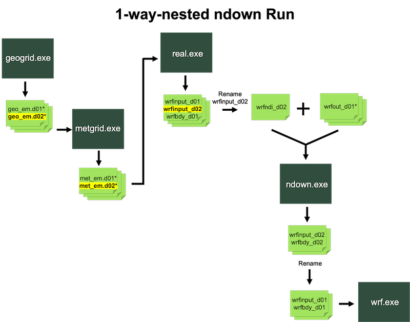
The ndown program is a tool used to run one-way nesting when the finer-grid-resolution domain is run subsequently after the coarser-grid-resolution run. The ndown.exe executable (manufactured during the WRF compile) is run in between the two simulations. The initial and lateral boundary conditions for the finer-grid run are obtained from the coarse grid run, with input from higher resolution terrestrial fields (e.g. terrain, landuse, etc.), and masked surface fields (such as soil temperature and moisture). The ndown program can be useful for the following scenarios.

• When a long simulation (e.g., several years) has already been run, and it is later decided to embed a nest with higher-resolution.

• When there are multiple nests and the number of grid points in the finer-resolution domain(s) is much greater than the number of points in the parent domain(s). It is likely that more processors are needed to simulate the larger domains, while it is not possible to use too many processors for the smaller domain(s) (an error will occur). In this case, it may be necessary to use ndown to run the domains separately. See the FAQ on choosing an appropriate number of processors for additional details.

Running Ndown

Note

Using ndown requires the code to be compiled for nesting.

1. Obtain output from a single coarse grid WRF simulation.

   • Frequent output (e.g. hourly) from the coarse grid run is recommended to provide better boundary specifications.

   
   

2. Run geogrid.exe and metgrid.exe for two domains.

   
   

3. Run real.exe for 2 domains.

   • The purpose of this step is to ingest higher resolution terrestrial fields and corresponding land-water masked soil fields.

   • Copy or link the met_em* files to the directory in which you are running real.exe. For e.g.,

     ln -sf <path-to-WPS-directory>/met_em* .
     

   • Edit namelist.input. Set max_dom=2, making sure columns 1 and 2 are set-up for a 2 domain run (edit the correct start time and grid dimensions).

   • Run real.exe. This produces files: wrfinput_d01, wrfinput_d02, and wrfbdy_d01

   
   

4. Run ndown.exe to create the final fine-grid initial and boundary condition files.

   • Rename wrfinput_d02 to wrfndi_d02

     mv wrfinput_d02 wrfndi_d02
     

   • Modify and check the following namelist.input parameters.

     • Add io_form_auxinput2=2 to the &time_control record.

     • interval_seconds should reflect the history output interval from the coarse domain model run.

     • Set max_dom=2.

     • Do not change physics options until after running the ndown program.

     • (Optional) To refine the vertical resolution when running ndown, set vert_refine_fact (see Namelist Variables for details). Alternatively, use the utility v_interp to refine vertical resolution (see WRF Post-processing, Utilities, & Tools for details).

   • Run ndown.exe, which uses input from the coarse grid wrfout* file(s), and the wrfndi_d02 file. This produces files: wrfinput_d02 and wrfbdy_d02

     ./ndown.exe >& ndown.out
            or
     mpiexec -np 4 ./ndown.exe
     

   
   

5. Run the fine-grid WRF simulation.

   • Rename wrfinput_d02 to wrfinput_d01 and wrfbdy_d02 to wrfbdy_d01

     mv wrfinput_d02 wrfinput_d01
     mv wrfbdy_d02 wrfbdy_d01
     

   • Rename (or move) the original wrfout_d01* files so as to not overwrite them.

   • Modify and check the following namelist.input parameters.

     • Move the fine-grid domain settings for e_we, e_sn, dx, and dy from column 2 to column 1 so that this run is for the fine-grid domain only.

     • Set time_step to comply with the fine-grid domain (typically 6*DX).

     • Set max_dom=1

     • (Optional) At this stage, the WRF model’s physics options may be modified from those used for the initial single domain run, with the exception of the land surface scheme (sf_surface_physics) which has different numbers of soil depths depending on the scheme.

     • (Optional) To allow the initial and lateral boundaries to use the moist and scalar arrays, set have_bcs_moist=.true. and have_bcs_scalar=.true. - this option should only be used during wrf.exe, after the ndown process, and microphysics options must remain the same between forecasts. The advantage of this option is the parent domain simulation provides realistic lateral boundary tendencies for all microphysical variables, instead of a simple zero inflow or zero gradient outflow.

   • Run WRF for this grid.

Although output from this run (wrfout_d01*) uses the d01 domain ID, it is actually the output for the fine-resolution domain. It may help to rename these to avoid future confusion.

Running ndown for Three or more Domains

Ndown can be used for more than one nest, but the procedure is a bit cumbersome. Because of the way the code it written, it expects specific file names (specifically for d01 and d02), and therefore it is important to follow these steps precisely:

Note

This example is for nesting down to a 3rd domain (3 domains total), and assumes the wrfout_d01* files are already created.

1. Run the geogrid.exe and metgrid.exe programs for 3 domains.

   
   

2. Run real.exe for 3 domains.

   • Link or copy the met_em* files into the directory in which you are running real.exe.

   • In namelist.input, set max_dom=3, making sure columns 1, 2 and 3 are set-up for a 3-domain run (edit the correct start time and grid dimensions).

   • Run real.exe. This produces files: wrfinput_d01, wrfinput_d02, wrfinput_d03, and wrfbdy_d01.

   
   

3. Create the domain 02 initial and boundary condition files, by running ndown.exe (see details in section above).

   
   

4. Run the domain 2 WRF simulation (see details in the section above). After, wrfout_d01* files should be available. Though these files use the d01 domain ID, they actually correspond to domain 02.

   
   

5. Make the domain 03 initial and boundary condition files, by running ndown.exe.

   • Rename wrfinput_d03 to wrfndi_d02 (this is the name the program expects)

   • Modify and check the following namelist.input parameters.

     • Set io_form_auxinput2 = 2 in the &time_control record.

     • Set interval_seconds to reflect the history output interval from the coarse domain model run.

     • Set max_dom=2.

     • Move the values for i_parent_start and j_parent_start from column 3 to column 2. Keep the value set to =1 for column 1.

     • Do not change physics options until after running the ndown program.

     • Run ndown.exe, which uses input from the (new) coarse grid wrfout file(s), and the wrfndi_d02 file. This produces a wrfinput_d02 and wrfbdy_d02 file (both which will actually correspond to domain 03).

   
   

6. Make the fine-grid (d03) WRF run.

   • Rename “wrfinput_d02 to wrfinput_d01.

   • Rename wrfbdy_d02 to wrfbdy_d01.

   • Rename (or move) the wrfout_d01* files so as to not overwrite them (recall that these files correspond to d02).

   • Modify and check the following namelist.input parameters.

     • Move the fine-grid domain settings for e_we, e_sn, dx, and dy from the original column 3 (domain 03) to column 1 (domain 01) so that this run is for the fine-grid domain only.

     • Set time_step to comply with the fine-grid domain (typically 6*DX).

     • Set max_dom=1.

After running wrf.exe, you will have new wrfout_d01* files. These correspond to domain 03. If you need to add any more nests, follow the same format, keeping the naming convention the same (always using d01 and d02).

The following figure summarizes data flow for a one-way nested run using the ndown program.

Automatic Moving Nests (Vortex-following)

The automatic moving nest (or vortex-following) option tracks the center of low pressure in a tropical cyclone, and allows the nested domain to move inside the parent as the cyclone moves. Tropical cyclones typically move over a relatively large surface area over a relatively short time period. This option eliminates the need to use a large high-resolution nest (which can be computationally expensive), and tracks the cyclone as it moves inside its parent (coarse) domain.

To use this option, the WRF code must be configured and compiled with the vortex-following nesting option (option 3), in addition to the distributed-memory parallelization option (dmpar) to make use of multiple processors.

Note

• WRF compiled for vortex-following does not support the “specified move” or static nested (“basic”) options.

• No nest input is needed, but note that the automatic moving nest works best for a well-developed vortex.

To use non-default values, add and edit the following namelist variables in the &domains record:

vortex_interval	how often WRF calculates the vortex position, in minutes (default is 15 minutes)
max_vortex_speed	used with vortex_interval to compute the search radius for the new vortex center position (default is 40 m/sec)
corral_dist	the closest distance in the number of coarse grid cells between the moving nest boundary and the parent domain boundary (default is 8) - useful when there are more than two total domains (including the coarsest domain). This means, for e.g., the border of d03 is allowed to get to corral_dist* grid cells from any wall of its parent (d02), before the parent is forced to move. Note that d01 cannot move. This parameter can be used to center the telescoped nests so that all nests are moved together with the storm.
track_level	the pressure level (in Pa) where the vortex is tracked
time_to_move	the time (in minutes) until the nest is moved. This option may help when the storm is still too weak to be tracked by the algorithm.

When the automatic moving nest is employed, the model writes the vortex center location, with minimum mean sea-level pressure and maximum 10-m winds to the standard-out file (e.g. rsl.out.0000). Type the following command to produce a list of storm information at 15-minute intervals:

grep ATCF rsl.out.0000

which produces something similar to:

ATCF    2007-08-20_12:00:00            20.37   -81.80     929.7 133.9 |br|
ATCF    2007-08-20_12:15:00            20.29   -81.76     929.3 133.2

The initial location of the nest is specified through i_parent_start and j_parent_start in namelist.input.

Using high-resolution terrain and landuse with vortex-following

To incorporate high-resolution terrain and landuse input in a moving nest run (see Chen et al., 2007):

1. Set the folowing prior to configuring and compiling WRF (this example is for a ‘bash’ shell environment).

   export TERRAIN_AND_LANDUSE=1
   

   
   

2. By default, the WPS program uses MODIS landuse data, but the high-resolution data set specific to this option is from USGS. Therefore, to use this option, landuse data should be prepared using USGS static fields. Before running geogrid.exe, in the namelist.wps &domains record, set

   geog_data_res = 'usgs_30s+default'
   

   
   

3. Set the following in the &time_control record of namelist.input prior to running real.exe and wrf.exe.

   input_from_hires = .true., .true.,
   rsmas_data_path  = 'terrain_and_landuse_data_directory'
   

   
   

   Note

   This option overwrites the input_from_file namelist setting for nest domains.

Specified Moving Nests

The specified moving nest option allows you to dictate exactly where the nest moves; however, it can be quite intricate to set up and comes with the following stipulations:

• WRF must be configured and compiled with the preset moves nesting option (option 2), and configured for distributed-memory parallelization (dmpar) to make use of multiple processors.

• Only coarse grid input files are required since nest initialization is defined from the coarse grid data.

• In addition to standard nesting namelist options, the following must be added to the &domains section of namelis.input

Note

Code compiled with the “preset moves” option will not support static nested runs or the vortex-following option.

num_moves	the total number of moves during the model run. A move of any domain is counted toward this total. The maximum is currently set to 50, but can be changed by modifying MAX_MOVES in frame/module_driver_constants.F (and then recompiling the code to reflect the change, but neither a clean -a nor reconfiguration is necessary).
move_id	a list of nest IDs (one per move) indicating which domain moves for any given move
move_interval	the number of minutes from the beginning of the run until the first move occurs. The nest will move on the next time step after the specified interval has passed.
move_cd_x move_cd_y	distance in the number of grid points and direction of the nest move (positive numbers indicate moving toward east and north, while negative numbers indicate moving toward west and south)

Run-time Capabilities

WRF includes special run-time options. For a full list of options, see the namelist.input file options. Scroll down, or click of the topics below to learn more about the runtime options

• SST Update

• Adaptive Time-stepping

• Stochastic Parameterization Schemes

• Nudging in WRF

• Digital Filter Initialization

• Bucket Options

• Global Simulations

• I/O Quilting

SST Update

Most first-guess input data include an SST and sea-ice field, which is used to initialize the model and is usually sufficient for short simulations (less than five days) since ocean temperatures do not change quickly. However, because most WRF physics schemes do not predict sea-surface temperature (SST), vegetation fraction, albedo or sea ice, for simulations five or more days, it is recommended to use the sst_update option to read-in additional time-varying data and update these fields.

To use this option, users must obtain additional time-varying SST and sea ice fields to be processed during WPS. Twelve monthly values of vegetation fraction and albedo are already processed during the geogrid program. After WPS is complete, set the following options in the namelist.input &time_control record before running real.exe and wrf.exe:

io_form_auxinput4 = 2
auxinput4_inname = "wrflowinp_d<domain>"
auxinput4_interval = 360, 360, 360

and in the &physics record:

sst_update = 1

The real.exe program creates the wrflowinp_d<domain> file, in addition to wrfinput_d0** and wrfbdy_d01.

Note

sst_update cannot be used with sf_ocean_physics or vortex-following options.

Adaptive Time-stepping

Adaptive time stepping is a method to maximize the WRF model time step, while maintaining numerical stablity. Model time step is adjusted based on the domain-wide horizontal and vertical stability criterion (the Courant-Friedrichs-Lewy (CFL) condition). The following set of values typically work well:

• use_adaptive_time_step = .true.

  
  

• step_to_output_time = .true.

  Note that nest domain output still may not write at the correct time. If this happens, try using adjust_output_times = .true. to correct this

• target_cfl = 1.2, 1.2, 1.2 (max_dom)

  
  

• max_step_increase_pct = 5, 51, 51 (max_dom)

  A large percentage value for the nest allows the nested time step more freedom to adjust

• starting_time_step = -1, -1, -1 (max_dom)

  The default value “-1” means 4*DX at start time

• max_time_step = -1, -1, -1 (max_dom)

  The default value “-1” means 8*DX at start time

• min_time_step = -1, -1, -1 (max_dom)

  The default value “-1” means 3*DX at start time

• adaptation_domain=

  An integer value indicating which domain is driving the adaptive time step

See Namelist Variables for additional information on these options.

Stochastic Parameterization Schemes

WRF Stochastic Parameterization

Parameterization schemes used to represent model uncertainty in ensemble simulations by applying a small perturbation at every time step, to each member

The stochastic parameterization suite comprises a number of stochastic parameterization schemes, some widely used and some developed for very specific applications. Each scheme generates its own random perturbation field, characterized by spatial and temporal correlations and an overall perturbation amplitude, defined in the &stoch namelist.input record.

Random perturbations are generated on the parent domain at every time step and, by default, interpolated to the nested domain(s). The namelist settings determine on which domains these perturbations are applied. For e.g., by setting sppt=0,1,1, perturbations are applied on the nested domains (d02 and d03) only.

Since the scheme uses Fast Fourier Transforms (FFTs; provided in the library FFTPACK), the recommended number of gridpoints in each direction is a product of small primes. Using a large prime in at least one direction may substantially increase computational cost.

Note

• All below options are set in an added &stoch” namelist.input record

• max_dom indicates a value is needed for each domain

Random Perturbation Field

This option generates a 3-D Gaussian random perturbation field for user-implemented applications.

Activate this option by setting (max_dom):

rand_perturb=1,1

The perturbation field is saved in the history files (wrfout*) as rand_pert.

Stochastically Perturbed Physics Tendencies (SPPT)

A random pattern perturbs accumulated physics tendencies (except those from microphysics) of:

• potential temperature

• wind, and

• humidity

For details on the WRF implementation see Berner et al., 2015. Activate this option by setting (max_dom):

sppt=1,1

The perturbation field is saved in the history files (wrfout*) as rstoch.

Stochastic Kinetic-Energy Backscatter Scheme (SKEBS)

A random pattern perturbs:

• potential temperature, and

• the rotational wind component

Wind perturbations are proportional to the square root of the kinetic-energy backscatter rate, and temperature perturbations are proportional to the potential energy backscatter rate. For details on the WRF implementation see Berner et al., 2011 and WRF Implementation Details and Version history of a Stochastic Kinetic-Energy Backscatter Scheme (SKEBS). Default parameters are for synoptic-scale perturbations in the mid-latitudes. Tuning strategies are discussed in Romine et al. 2014 and Ha et al. 2015.

Activate this option by setting (max_dom):

skebs=1,1

The perturbation fields are saved in the history files as:

• ru_tendf_stoch* (for u)

• rv_tendf_stoch (for v)

• rt_tendf_stoch (for θ)

Stochastically Perturbed Parameter Scheme (SPP)

A random pattern perturbs parameters in the following selected physics packages:

• GF convection scheme

• MYNN boundary layer scheme

• RUC LSM

Activate this option by setting (max_dom):

spp=1,1

Parameter perturbations to a single physics package can be achieved by setting spp_conv=1, spp_pbl=1, or spp_lsm=1. For implementation details see Jankov et al..

The perturbation field is saved in the history files (wrfout*) as:

• pattern_spp_conv*

• pattern_spp_pbl*

• pattern_spp_lsm*

Stochastic Perturbations to the Boundary Conditions (perturb_bdy)

The following two options are available:

• perturb_bdy=1

  The stochastic random field perturbs the boundary tendencies for wind and potential temperature. This option runs independently of SKEBS (skebs=1) and may be run with or without setting skebs=1, which operates solely on the interior grid. Note that this option requires the generation of a domain-size random array, thus computation time may increase.

• perturb_bdy=2

  A user-provided pattern perturbs the boundary tendencies. Arrays are initialized and called: field_u_tend_perturb, field_v_tend_perturb, and field_t_tend_perturb. These arrays should be filled with the desired pattern in spec_bdytend_perturb in the share/module_bc.F file or spec_bdy_dry_perturb in the dyn_em/module_bc_em.F file. Once these files are modified, WRF must be recompiled (but neither a clean -a nor a reconfigure are necessary).

Stochastic perturbations to the boundary tendencies in WRF-CHEM (perturb_chem_bdy)

A random pattern perturbs the chemistry boundary tendencies in WRF-Chem. For this application, WRF-Chem must be compiled at the time of the WRF compilation.

Activate this option by setting (max_dom):

rand_perturb=1,1

The perturb_chem_bdy option runs independently of rand_perturb and therefore may be run with or without the “rand_perturb” scheme, which operates solely on the interior grid. However, perturb_bdy_chem=1 requires the generation of a domain-sized random array to apply perturbations in the lateral boundary zone, thus computation time may increase. When running WRF-Chem with have_bcs_chem=.true. in the &chem namelist.input record, chemical LBCs read from wrfbdy_d01 are perturbed with the random pattern created by rand_perturb=1.

WRF-Solar stochastic ensemble prediction system (WRF-Solar EPS)

WRF-Solar includes a stochastic ensemble prediction system (WRF-Solar EPS) tailored for solar energy applications (Yang et al., 2021; Kim et al., 2022). The stochastic perturbations can be introduced into variables of six parameterizations, controlling cloud and radiation processes. See details of the model on the WRF-Solar EPS website. See Namelist Variables in the &stoch section.

Nudging in WRF

KKW add overall ‘nudging’ section and then put the diff types under that. put definitions of types at the top in containers. put this note in the top section:

Note

The DFI option can not be used with nudging options.

Analysis/Grid Nudging (Upper-air and/or Surface)

Analysis Nudging

A method to nudge the WRF model toward data analysis for coarse-resolution domains

The model is run with extra nudging terms for horizontal winds, temperature, and water vapor. These terms nudge point-by-point to a 3d space- and time-interpolated analysis field.

Using Analysis Nudging

1. Use WPS to prepare input data for WRF, as usual.

   • If nudging is desired in the nest domains, make sure all time periods for all domains are processed in WPS.

   • If using surface-analysis nudging, the OBSGRID tool must be run after metgrid. OBSGRID outputs a wrfsfdda_d01 file, which is required by the WRF model when using this option.

   
   

2. Set the following options in &fdda in namelist.input before running real.exe. (max_dom) indicates a value should be set for each domain you wish to nudge.

   
   

   grid_fdda=1	turns on analysis nudging (max_dom)
   gfdda_inname=’wrffdda_d<domain>’	the defined name of the file the real program will write out
   gfdda_interval_m	time interval of input data in minutes (max_dom)
   gfdda_end_h	end time of grid-nudging in hours (max_dom)

   
   
   
   

   The following additional options can be set (see examples.namelist in the test/em_real directory of the WRF code for details):

   
   

   io_form_gfdda=2	analysis data I/O format (2=netcdf)
   fgdt	calculation frequency (mins) for grid-nudging (0=every time step; (max_dom))
   if_no_pbl_nudging_uv	1=no nudging of u and v in the PBL, 0=nudging in the PBL (max_dom)
   if_no_pbl_nudging_t	1=no nudging of temperature in the PBL, 0=nudging in the PBL (max_dom)
   if_no_pbl_nudging_q	1=no nudging of qvapor in the PBL, 0=nudging in the PBL (max_dom)
   guv=0.0003	nudging coefficient for u and v (sec-1) (max_dom)
   gt=0.0003	nudging coefficient for temperature (sec-1) (max_dom)
   gq=0.00001	nudging coefficient for qvapor (sec-1) (max_dom)
   if_ramping	0=nudging ends as a step function; 1=ramping nudging down at the end of the period
   dtramp_min	time (mins) for the ramping function (if_ramping)

   
   
   
   

   If doing surface analysis nudging, set:

   
   

   grid_sfdda=1	turns on surface analysis nudging (max_dom)
   sgfdda_inname=”wrfsfdda_d<domain>”	This is the defined name of the input file from OBSGRID.
   sgfdda_interval_m	time interval of input data in minutes
   sgfdda_end_h	end time of surface grid-nudging in hours

   
   
   
   

   An alternative surface data nudging option nudges surface air temperature and water vapor mixing ratio (as with grid_sfdda=1), but uses tendencies generated from the direct nudging approach to constrain surface sensible and latent heat fluxes, thus ensuring thermodynamic consistency between the atmosphere and land surface. This option works with the YSU PBL and the Noah LSM. (Alapaty et al., 2008). To use this option, set:

   
   

   • grid_sfdda=2

   
   

3. Run real.exe, which, in addition to the wrfinput_d0* and wrfbdy_d01 files, will create a wrffdda_d0* file that is then used by wrf.exe.

Note

For additional guidance, see Steps to Run Analysis Nudging, along with the test/em_real/examples.namelist file provided with the WRF code.

Spectral Nudging

Spectral Nudging

An upper-air nudging option that selectively nudges only the coarser scales, and is otherwise set up similarly to grid-nudging, but additionally nudges geopotential height.

Set the following namelist.input parameters to use this option. Note that max_dom indicates a value should be set for each domain:

grid_fdda=2	turns on spectral nudging option (max_dom)
xwavenum = 3	defines the number of waves contained in the domain in the x-direction; this is the maximum wave that is nudged
ywavenum = 3	defines the number of waves contained in the domain in the y-direction; this is the maximum wave that is nudged

Observational Nudging

Observational Nudging

A method to nudge the WRF model toward observations

When using this option, similar to Analysis/Grid Nudging (Upper-air and/or Surface), the model is run with extra nudging terms for horizontal winds, temperature, and water vapor; however, in obs-nudging, points near observations are nudged based on model error at the observation site. This option is suitable for fine-scale or asynoptic observations. See the Observation Nudging Users Guide, Experimental Nudging Options, and README.obs_fdda in WRF/test/em_real/ for details.

Using Observational Nudging

In addition to the standard WPS preparation of input data, station observation files are required, and must be prepared using the OBSGRID program, which outputs files OBS_DOMAIN10* for domain 1, and OBS_DOMAIN20* for domain 2, etc. Once these files are created, they must all be concatenated into a single file per domain, with the naming convection, for e.g., for d01, OBS_DOMAIN101.

Observation nudging is then activated during WRF, using the following namelist settings in the &fdda record. Note that (max_dom) indicates the setting should be applied to each domain you wish to nudge.

obs_nudge_opt=1	turns on observational nudging (max_dom)
fdda_start	obs nudging start time in minutes (max_dom)
fdda_end	obs nudging end time in minutes (max_dom)

And the following should be set in the &time_control record:

auxinput11_interval_s

interval in seconds for observation data; set to an interval small enough to include all observations

Below are additional namelist options (set in the &fdda record):

max_obs=150000	The maximum number of observations used on a domain during any given time window
obs_nudge_wind	set to 1 to nudge wind, 0=off (max_dom)
obs_coef_wind=6.E-4	nudging coefficient for wind (s-1) (max_dom)
obs_nudge_temp	set to 1 to nudge temperature, 0=off (max_dom)
obs_coef_temp=6.E-4	nudging coefficient for temperature (s-1) (max_dom)
obs_nudge_mois	set to 1 to nudge water vapor mixing ratio, 0=off (max_dom)
obs_coef_mois=6.E-4	nudging coefficient for water vapor mixing ratio (s-1) (max_dom)
obs_rinxy=240.	horizontal radius of influence in km (max_dom)
obs_rinsig=0.1	vertical radius of influence in eta
obs_twindo=0.6666667	half-period time window over which an observation will be used for nudging, in hours (max_dom)
obs_npfi=10	frequency in coarse grid timesteps for diagnostic prints
obs_ionf=2	frequency in coarse grid timesteps for observational input and error calculation (max_dom)
obs_idynin	set to 1 to turn on the option to use a “ramp-down” function for dynamic initialization, to gradually turn off FDDA before the pure forecast
obs_dtramp=40.	time period in minutes over which nudging is ramped down from one to zero, when obs_idynin=1 is set
obs_prt_freq=10	frequency in obs index for diagnostic printout (max_dom)
obs_prt_max=1000	maximum allowed obs entries in diagnostic printout
obs_ipf_errob=.true.	true=print obs error diagnostics; false=off
obs_ipf_nudob=.true.	true=print obs nudge diagnostics; false=off
obs_ipf_in4dob=.true.	true=print obs input diagnostics; false=off

Note

For additional information and namelist options related to nudging, see the examples.namelists file in the WRF code’s test/em_real directory.

Digital Filter Initialization

Digital filter initialization (DFI) is a method to remove initial model imbalance as, for example, measured by the surface pressure tendency. This may be important if you are interested in the 0-6 hour simulation/forecast. It runs a digital filter during a short model integration, backward and forward, and then starts the forecast. In WRF implementation, this is all done in a single job. DFI can be used for multiple domains with concurrent nesting, with feedback disabled.

Using DFI

Prior to using the DFI option, there is no special requirement for data preparation. Run WPS per usual.

1. Open the example.namelist file residing in the test/em_real/ directory and find the &dfi_control section. Copy and paste that section into the namelist.input file, making edits to match the case configuration (e.g. dates). For a typical application, the following options are used:

   
   

   dfi_opt=3	which DFI option to use (0=no DFI; 1=digital filter launch; 2=diabatic DFI; 3=twice DFI - option 3 is recommended; Note: if doing a restart, this must be changed to 0)
   dfi_nfilter=7	which digital filter type to use (0=uniform; 1=Lanczos; 2=Hamming; 3=Blackman; 4=Kaiser; 5=Potter; 6=Dolph window; 7=Dolph; 8=recursive high-order - option 7 is recommended)
   dfi_cutoff_seconds=3600	cutoff period (in seconds) for the filter (should not be longer than the filter window)
   dfi_write_filtered_input=.true.	option to produce a filtered wrfinput file (“wrfinput_initialized_d01”) when running wrf.

   
   

   The following time specifications are typically set so that integration goes backward for 0.5 to 1 hour, and integration forward is for half that time.

   
   

   • dfi_bckstop_year
     dfi_bckstop_month
     dfi_bckstop_day
     dfi_bckstop_hour
     dfi_bckstop_minute
     dfi_bckstop_second

   
   

   • dfi_fwdstop_year
     dfi_fwdstop_month
     dfi_fwdstop_day
     dfi_fwdstop_hour
     dfi_fwdstop_minute
     dfi_fwdstop_second

• To use the constant boundary condition option, set constant_bc=.true. in the &bdy_control namelist record.

• If planning to use a different time step for DFI, it can be set with the time_step_dfi option.

Note

• The DFI option can not be used with nudging options.

• The DFI option can not be used with the multi_bdy_files=.true. option.

Bucket Options

WRF Bucket options are available to maintain accuracy in rainfall accumulation (RAINC, RAINNC) and/or radiation budget accumulation (ACSWUPT, ACLWDNBC) during months- to years-long simulations.

With 32-bit accuracy, adding small numbers to very large numbers causes a loss of accuracy as the accumulation term increases. For simulations of days to weeks, accumulations are usually okay, but for months to years, this can truncate the additions (particularly small ones may be zeroed-out). When bucket options are activated, part of the term is stored in an integer that increments by 1 each time the bucket value is reached.

Water Accumulation

In the &physics namelist record, set bucket_mm*, which is the bucket reset value for water accumulations (in mm). The following two terms are produced:

• RAINNC

• I_RAINNC

where RAINNC now only contains the remainder. The total is retrieved from the output using the following equation:

total = RAINNC + bucket_mm * I_RAINNC

A reasonable bucket value may be based on a monthly accumulation (e.g., 100 mm). Total precipitation is found with the equation:

total precipitation = RAINC + RAINNC, where

• Total RAINNC = RAINNC + bucket_mm * I_RAINNC

• Total RAINC = RAINC + bucket_mm * I_RAINC

Radiation Accumulation

In the &physics namelist record, set bucket_J, which is the bucket reset value for energy accumulations (in Joules). The radiation accumulation terms (e.g., ACSWUPT) are in Joules/m², so that the mean value over a simulation period is the difference divided by the time between, giving W/m². The typical value, based on a monthly accumulation, is 1.e9 J. Here the total is given by the following (Note - this is an example for the term ACSWUPT - other radiative terms follow the same equation concept):

total = ACSWUPT+bucket_J*I_ACSWUPT

Global Simulations

Note

For global simulations, users are encouraged to use the NSF NCAR MPAS model instead of WRF.

Although WRF supports modeling a global domain, the option is not commonly-used or tested. Not all physics and diffusion options have been tested with it, and some options may not work well with polar filters. Positive-definite and monotonic advection options do not work with polar filters in a global run because polar filters can generate negative values of scalars (which implies that WRF-Chem cannot be run with positive-definite and monotonic options in a global WRF setup).

Using a Global Domain

1. Run WPS, starting with the namelist template namelist.wps.global.

   • Set map_proj=’lat-lon’, and grid dimensions e_we and e_sn. Save the file.

   • There is no need to set dx and dy. The geogrid program calculates grid distances whose values can be found in the global attribute section of geogrid output files (e.g., geo_em.d01.nc).

   • Run geogrid.exe.

   • Use the command ncdump -h geo_em.d01.nc to see the grid distances, which must later be used for dx and dy values in WRF’s namelist.input file. Grid distances in the x and y directions may be different, but it is best that they are set similarly or the same. WRF and WPS assume the earth is a sphere, with a radius of 6370 km. There are no restrictions on what to use for grid dimensions, but for effective use of the polar filter in WRF, the east-west dimension should be set to 2P*3Q*5R+1 (where P, Q, and R are any integers, including 0).

   • Run the remaining WPS programs as usual, but for only one time period. Because the domain covers the entire globe, lateral boundary conditions are not needed.

   
   

2. Run real.exe for only a single time period. The lateral boundary file wrfbdy_d01 is not needed.

3. Copy namelist.input.global to namelist.input, then edit it specific to the configuration.

4. Run wrf.exe.

I/O Quilting

The I/O Quilting option reserves a few processors to manage output only, which can sometimes be performance-friendly if the domain size is very large, and/or the time taken to write each output is significant when compared to the time taken to integrate the model between output times.

Note

This option should be used with care, and only used if the user is highly experienced with computing processes.

To use quilting, the following parameters should be set in the &namelist_quilt record in namelist.input.:

• nio_tasks_per_group : Number of processors to use per IO group for IO quilting (1 or 2 is typically sufficient)

• nio_groups : How many IO groups for IO (default is 1)

Note

This option is only available for use with wrf.exe. It does not work for real or ndown.