WRF Software & Computation¶

WRF Build Mechanism¶

The WRF build mechanism standardizes the WRF code building process for different types of computing environments/platforms. Its components and functions are described below. For instructions on building WRF, see Compiling.

Build Components¶

The build mechanism’s primary components consist of the following. Read below for details.

Scripts
Programs
Makefiles
Configuration Files
Registry
Environment Variables

Scripts¶

The top-level WRF/ directory contains three user-executable scripts:

configure (which relies on the Perl script WRF/arch/Config_new.pl)
compile
clean

Programs¶

A substantial portion of WRF code is automatically generated during the build. This is done by the tools/registry file.

Makefiles¶

Much of the WRF code is written in the C and C++ programming language. These languages utilize a command called “make,” which, when executed, performs the actions listed in a file called a Makefile. WRF contains a primary Makefile in its top-level directory (WRF/), and additional makefiles in various subdirectories. When WRF is built/compiled, make is called recursively over the directory structure.

Configuration Files¶

Prior to building/compiling WRF, a configure script is run. This script generates a configure.wrf file, which contains details about the compiler, linker, build settings, rules, and macro definitions used by the “make” utility. It is read by WRF Makefiles (except Makefiles in the WRF/tools and WRF/external directories). configure.wrf is deleted when the code system is cleaned by the user-issued clean script. Thus, configure.wrf can be modified for temporary changes, such as optimization levels and compiling with debugging. Permanent changes should be made in arch/configure_new.defaults. The configure.wrf file is composed by the following three files:

arch/configure_new.defaults : contains lists of compiler options for all supported platforms and configurations; changes made to this file are permanent
arch/preamble_new : constitutes the generic parts (non-architecture-specific) of the configure.wrf file; See the file for details.*
arch/postamble_new : similar to arch/preamble_new. See the file for details.

Registry¶

A Registry file contains defining aspects of variables used in the model, which are read and accounted for during a WRF code build/compile. Registry files are found in the WRF/Registry directory. The files are named Registry.x (or registry.x), where x is a specific application (e.g., Registry.EM_CHEM includes variables specific to the WRF Chemistry model). For a basic WRF build/compile, the file used is Registry.EM_COMMON, which contains shared entries for all applications.

As part of the WRF build/compile process, WRF/tools/registry* files look for a file named “Registry” to read as input. Prior to compiling the code, the configure script is run to incorporate user-specified applications. Based on these specifications, configure copies the appropriate Registry.x file to the expected file name Registry.

Important

Because the Registry file is created during the build/compile, if any modifications are made to it, they will be lost during the compile. Modifications should be made to the Registry.x files.

Environment Variables¶

An environment variable is user-defined (or defined by the user’s computing environment), and determines computation specifics. For WRF configure and compile processes, environment variables determine the following:

Location of the netCDF library and Perl command
Which WRF dynamic core to compile
Machine-specific features
Optional build libraries (such as Grib Edition 2, HDF, and parallel netCDF)

In addition to WRF-related environment settings, there may also be settings specific to particular compilers or libraries. For e.g., local installations may require setting a variable like MPICH_F90 to ensure the correct instance of the Fortran 90 compiler is used by the mpif90 command.

WRF Build Mechanics¶

The two steps in the WRF build process are configuration and compilation.

Configuration¶

The configure script (in the top-level WRF directory) configures the model to determine information about the user’s computing environment prior to compilation, and it steps through the following processes:

Tries to locate mandatory and optional libraries (e.g., netCDF or HDF) and tools (e.g., Perl); it checks for these in standard paths, or paths from the user’s shell environment settings
Calls the UNIX “uname” command to determine the user’s platform
The Perl script arch/Config_new.pl is executed, displaying a list of available machine configurations for the user to choose from
The user-selected set of options is then used to generate the configure.wrf file in the top-level directory

Note

Each time the clean script is used, the configure.wrf file is overwritted, but is saved as configure.wrf.backup.

Compilation¶

The compile script (located in the top-level WRF directory) steps through the processes to build/compile the WRF code after it has been configured. It performs checks, creates an argument list, copies the appropriate Registry.X file to Registry/Registry (see Registry). The script then issues the UNIX “make” command, using the Makefile in the top-level WRF/ directory, along with recursive invocations of “make” in the WRF subdirectories, and configure.wrf’s settings to build the WRF code. The order of a complete build is as follows:

make is issued from the WRF/external directory
- make is issued from WRF/external/io_{grib1,grib_share,int,netcdf} for Grib Edition 1, binary, and netCDF implementations of I/O API
- make is issued from WRF/external/RSL_LITE to build the communications layer (distributed-memory/dmpar builds only)
- make is issued from WRF/external/esmf_time_f90 to build the ESMF time manager library
- make is issued from WRF/external/fftpack to build the FFT library for the global filters
- make is issued from other WRF/external directories, as specified by the “external:” target in configure.wrf
make is issued from the WRF/tools directory to build the program that reads the WRF/Registry/Registry file and auto-generate files in the WRF/inc directory
make is issued from the WRF/frame directory to build the WRF framework-specific modules
make is issued from the WRF/share directory to build the mediation layer routines, including WRF I/O modules that call the I/O API
make is issued from the WRF/phys directory to build the WRF model layer routines for physics
make is issued from the WRF/dyn_em directory to build mediation-layer and model-layer subroutines
make is issued from the WRF/main directory to build the WRF’s main programs, which are symbolically linked to a location based on the build case argument to the compile script (e.g., for a real-data case, the executables are linked to WRF/test/em_real)
- Source files (*.F or *.F90 files) are preprocessed to produce *.f90 files, which are input to the compiler. Registry-generated files from the WRF/inc directory may be included.
- *.f90 files are compiled, which creates object files (*.o) that are added to the library WRF/main/libwrflib.a. Most WRF/external/* directories generate their own library file.
- Executables are generated - depending whether an idealized or real-data case is chosen in the case argument to the compile command, the following are built:
  - Idealized Case
    - wrf.exe (the WRF model executable)
    - ideal.exe (a preprocessor for idealized cases)
  - Real-data Case
    - wrf.exe (the WRF model executable)
    - real.exe (a preprocessor for real-data cases)
    - ndown.exe (for one-way nesting)
    - tc.exe (for tropical storm addition or removal)

Note

The *.o files and *.f90 files created during the compile are kept until the WRF/clean script is used. When runtime errors refer to line numbers, or when using debugging tools (e.g., dbx or gbd), the line numbers are specific to the *.f90. However, code changes should be made to the *.F files.

Registry¶

Registry

A system that includes a Registry program that builds WRF code according to the Registry file, which contains a text-based table that lists and describes state fields and their attributes.

The WRF code is largely generated from the Registry, which provides a high-level, single-point of control over the fundamental structure of the model data. The Registry consists of two components:

Registry file (in WRF/Registry)
Registry program (in WRF/tools).

The WRF/Registry directory contains the following files:

File Name	Type of WRF Build
Registry.EM_COMMON	Standard/Basic WRF; containing variables common to all applications
Registry.EM_COMMON.var	Minimal subset of Registry.EM_COMMON required for a WRFDA compile
Registry.EM_CHEM	WRF Chemistry (WRF-Chem)
Registry.wrfvar	WRF Data Assimilation (WRFDA)
Registry.wrfchemvar	WRF-Chem + WRFDA
Registry.tladj	WRFPLUS

The Registry.X files define:

Variables
- Input or output fields
- Fields required for parallel communication
- Fields associated with a specific physics package
- Fields that provide tendencies to multiple physics or dynamics routines
Communication
Namelist options

The following attributes are declared for each state variable listed in the Registry.X file:

Variable name
Dimensionality
WRF I/O behavior and streams
Horizontal and vertical staggering
Feedback and nesting interpolation requirements

The Registry file provides input to generate communications for distributed memory processing (halo exchanges between patches, support for periodic lateral boundaries, and array transposes for FFTs to be run in the X, Y, or Z directions). The Registry associates various fields with particular physics packages, preventing over-allocation.

Registry Mechanics¶

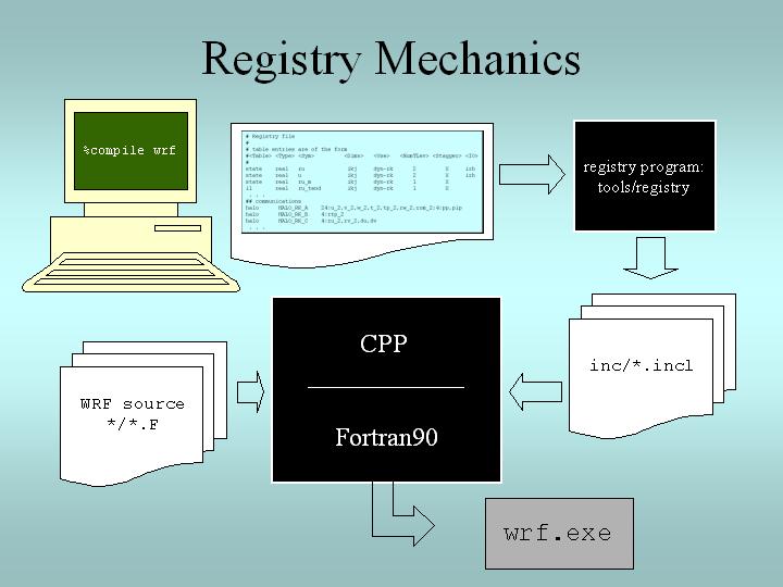
When a WRF build is initiated, the appropriate Registry.X file is copied to a file named Registry. The Registry program/executable (written in C and found in WRF/tools) uses the contents of the Registry file to generate files in the WRF/inc directory. These “include” files are used by the WRF Fortran source files during compilation. The Registry is used to build all model executables. Refer to the below image for details:

"An image that shows when the user compiles WRF, the Registry Program reads Registry/Registry, producing auto-generated sections of code that are stored in files in the inc directory. These are included into WRF using the CPP preprocessor and the Fortran compiler."

Registry Entries¶

The following entry types are used in the WRF Registry.X file:

Dimspec	Dimensions used to define arrays in the model
State	State variables and arrays in the domain structure
i1	Local variables and arrays in WRF’s “solve” routine (WRF/dyn_em/solve_em.F)
Typedef	Derived types that are subtypes of the domain structure
Rconfig	Represents namelist variables or arrays
Package	Packaged attributes (e.g. for a specific physics package)
Halo	Halo update interprocessor communications
Period	Communications for periodic boundary updates
Xpose	Communications for parallel matrix transposes
include	Similar to a CPP #include file

Dimspec¶

Dimspec

Registry file entries that consist of dimension specifications of WRF fields.

The below example assigns dimension names to the i, j, and k dimensions:

<Table>  <Dim>  <Order> <How defined>  <Coord-axis>  <Dimname in Data sets>
dimspec    i      1     standard_domain     x          west_east
dimspec    j      3     standard_domain     y          south_north
dimspec    k      2     standard_domain     z          bottom_top

Tip

Use the ncdump -h command to list the variables found in a WRF output/history file. For each variable, the three directional dimensions appear as west_east, south_north, and bottom_top.

Miscellaneous Dimspec Notes:

Because WRF uses horizontal and vertical staggering, dimension names include a _stag suffix, representing staggered sizes.
The list of names in the <Dim> column may either be a single/unique character, or a string with no embedded spaces (e.g., my_dim).
When this dimension is used within the Registry for State and I1 Variables, it must be surrounded by curly braces (e.g., {my_dim}).
The <Dim> variable is not case specific.
To keep the WRF system consistent between build types, a unified registry.dimspec file is used (located in the Registry directory), and is included in each Registry.* file.

State and I1 Variables¶

state Variable

A field eligible for input/output (I/O) and communications, and exists for the duration of the model forecast.

i1 Variable

“Intermediate level one” fields - typically tendency terms computed during a single model time-step, and then discarded prior to the next time-step.

Note

For i1 variables, space allocation and de-allocation is automatic (part of the model’s “solver” stack).

Below are the columns (in order from left to right) used for state and i1 variables in the Registry file.

Column Heading	Description	Type
Table	either state or i1	string
Type	type of variable or array	real, double, integer, logical, character, or derived
Sym	symbolic name inside WRF	string; not case-sensitive
Dims	dimensionality of the array	string; use hyphen (-) when dimensionless
Use	denotes association with the solver (dyn_em), or 4D scalar array	string; if not specific, declared misc
NumTLev	number of time levels	integer for arrays; use hyphen (-) for variables
Stagger	indicates staggered dimensions	string; X,Y,Z, or hyphen (-) if not staggered
IO	whether and how it is subject to I/O and nesting	string; use hyphen (-) when no specification
Dname	metadata name	string; in quotes
Descrip	metadata description	string; in quotes
Units	metadata units	string; in quotes

<Table> <Type> <Sym> <Dims>  <Use>  <NumTLev>  <Stagger> <IO> <DNAME>  <DESCRIP>             <UNITS>
state    real   u_gc   igj     dyn_em     1        XZ       i1   "UU"    "x-wind component"    "m s-1"

In this above example, the column descriptions indicate that this variable:

Is a state variable (<Table>)
Is a Fortran type “real” (<Type>)
Uses the field name u_gc in the model code (<Sym>)
Is a three-dimensional array igj (<Dims>)
Is used in association with the WRF solver (in WRF/dyn_em) (<Use>)
Has a single time level (<NumTLev>)
Is staggered in the X and Z directions (<Stagger>)
Is input only to the real program, i1 (<IO>)
Uses the field name UU in netCDF output files (<DNAME>)
Is described as the “x-wind component” (<DESCRIP>)
Has units of m/s (<UNITS>)

Note

The variable description (<DESCRIP>) and <UNITS> columns are used for post-processing purposes only.

Rconfig¶

rconfig

Run-time configuration (namelist.input) options defined in the Registry file

Each rconfig namelist option is described in its own line/row. Default values for each namelist variable are assigned in the Registry. The two below examples show the standard rconfig entry format:

<Table>  <Type>    <Sym>       <How set>              <Nentries>   <Default>
rconfig  integer   run_days    namelist,time_control        1           0
rconfig  integer   start_year  namelist,time_control   max_domains    1993

Where each column is described below:

Column Heading	Description	Notes
Table	entry type	‘rconfig’
Type	type of variable or array	real, integer, logical
Sym	symbolic name inside WRF	string; not case-sensitive
How set	namelist,<fortran record>	string
Nentries	dimensionality (# of entries)	either ‘1’ (single entry valid for all domains) or ‘max_domains’ (value specified for each domain)
Default	default setting for the variable	if entry is missing from namelist, this value is used

Note

Each namelist variable is a member of one of the specific namelist records. The previous example shows that run_days and start_year are both members of the time_control record.

The registry program constructs two subroutines for each namelist variable: one to retrieve the value of the namelist variable, and the other to set the value. For an integer variable named my_nml_var, the following code snippet provides an example of the easy access to the namelist variables:

INTEGER :: my_nml_var, dom_id
CALL nl_get_my_nml_var ( dom_id , my_nml_var )

The subroutine takes two arguments. The first is the input integer domain identifier, dom_id, (for example, 1 for the most coarse grid, 2 for the second domain), and the second argument is the returned value of the namelist variable. The associated subroutine to set the namelist variable, with the same argument list, is nl_set_my_nml_var. For namelist variables that are scalars, the grid identifier should be set to 1.

The rconfig line may also be used to define variables that are convenient to pass around in the model, usually part of a derived configuration (such as the number of microphysics species associated with a physics package). In this case, the <How set> column entry is derived. This variable does not appear in the namelist, but is accessible with the same generated nl_set and nl_get subroutines.

Halo¶

Distributed memory, inter-processor communications are fully described in the Registry file. An entry in the Registry constructs a code segment which is included (with cpp) in the source code. Following is an example of a halo communication:

<Table>  <CommName>   <Core>   <Stencil:varlist>
halo      HALO_EM_D2_3 dyn_em    24:u_2,v_2,w_2,t_2,ph_2;24:moist,chem,scalar;4:mu_2,al

Below are the columns used for halos (printed in order from left to right in the Registry file).

Column Heading	Description	Notes
Table	entry type	‘halo’
CommName	communication	case-sensitive, starts with ‘HALO_EM’
Core	dynamical core	all are set to ‘dyn_em;’ no longer relevant since dyn_nmm is removed from WRF
Stencil:varlist	stencil size and variables communicated with that stencil size	portion prior to colon (:) is size; comma-separated list after defines variables;

Note

Different stencil sizes are available, and are separated in the same <Stencil:varlist> column by a semi-colon (;). Stencil sizes 8, 24, and 48 all refer to a square with an odd number of grid cells on a side, with the center grid cell removed (8 = 3x3-1, 24 = 5x5-1, 48 = 7x7-1). The special small stencil 4 is just a simple north, south, east, west communication pattern.

The WRF model provides a communication immediately after a variable has been updated. The communications are restricted to the mediation layer (an intermediate layer of the software placed between the framework and model levels). The model level is where developers spend most of their time. The majority of users will insert communications into the dyn_em/solve_em.F subroutine. The HALO_EM_D2_3 communication shown in the above example is activated by inserting a small section of code that includes an automatically-generated code segment into the solve routine, via standard cpp directives:

#ifdef DM_PARALLEL
#    include "HALO_EM_D2_3.inc"
#endif

Parallel communications are only required when the code is built for distributed-memory parallel processing, which accounts for the surrounding #ifdef.

Period¶

Period communications are required when periodic lateral boundary conditions are selected. The Registry syntax is very similar for period and halo communications, but here stencil size refers to how many grid cells to communicate, in a direction that is normal to the periodic boundary:

<Table>     <CommName>        <Core>   <Stencil:varlist>
period   PERIOD_EM_COUPLE_A    dyn_em    2:mub,mu_1,mu_2

Xpose¶

The xpose (a data transpose) entry is used when decomposed data is to be re-decomposed. This is required when doing FFTs in the x-direction for polar filtering, for example. No stencil size is necessary:

<Table>     <CommName>        <Core>      <Varlist>
xpose    XPOSE_POLAR_FILTER_T  dyn_em   t_2,t_xxx,dum_yyy

It is likely additions will be added to the the parallel communications portion of the Registry file (halo and period), but unlikely that additions will be added to xpose fields.

Package¶

The package option in the Registry file associates fields with particular physics packages. It is mandatory that all 4-D arrays be assigned. Any 4-D array not associated with the selected physics option at run-time is neither allocated, used for I/O, nor communicated. All other 2-D and 3-D arrays are eligible for use with a package assignment, but that is not required. The package option’s purpose is to allow users to reduce the memory used by the model, since only necessary fields are processed. An example for a microphysics scheme is given below:

<Table>  <PackageName>  <NMLAssociated>    <Variables>
package   kesslerscheme   mp_physics==1   - moist:qv,qc,qr

Column Heading	Description	Notes
Table	entry type	‘package’
PackageName	name of associated options for code IF/CASE statements	string
NMLAssociated	package is associated with these namelist options	namelist setting, using ‘==’ syntax
Variables	all variables included in the package	syntax is: dash (-), space, 4-D array name, colon (:), then comma-separated list of 3-D arrays constituting 4-D amalgamation

In the example above, the 4-D array is moist, and the selected 3-D arrays are qv, qc, and qr. If more than one 4-D array is required, a semi-colon (;) separates those sections from each other in the <Variables> column.

The package entry is also used to associate generic state variables, as shown in the example following. If the namelist variable use_wps_input is set to 1, then the variables u_gc and v_gc are available to be processed:

<Table>  <PackageName> <NMLAssociated>     <Variables>
package     realonly    use_wps_input==1  - state:u_gc,v_gc

Modifying the Registry¶

Each line entry in the Registry.X file is specific to a single variable; however, a single entry may be spread across several lines - each line ending with a backslash (), denoting the entry continues to the next line. When adding a new line to the Registry, keep in mind the following:

It is recommended to copy an entry that is similar to the new entry, and then modify the new entry.
The Registry is not sensitive to spatial formatting.
White space separates identifiers in each entry.
After any change to a registry file, the code must be cleaned, reconfigured, and recompiled.
If a column has no entry, do not leave it blank. Use the dash character ( - ).

Adding a variable into the model typically only requires the addition of a single line to the Registry.X file, regardless of dimensionality. The same is true when defining a new run-time option (i.e., a new namelist entry). As with the model state arrays and variables, the entire model configuration is described in the Registry. Since the Registry modifies code for compile-time options, any change to the Registry (i.e., any file in the Registry directory) requires the code to be returned to the original unbuilt status with the clean -a command, and then reconfigured and recompiled.

WRF Architecture¶

The WRF model architecture is divided into the following different layers:

Driver Layer

The WRF Driver is responsible for handling domains and their time loop. It allocates, stores, decomposes, and represents abstractly as single data objects. To handle time looping, there are algorithms for integration over nest hierarchy (see Timekeeping).

Mediation Layer

The mediation layer contains the Solve routine, which uses a sequence of calls to take a domain object and advance it one time step. It also controls nest forcing, interpolation, and feedback routines. It dereferences fields in calls to the physics dirvers and dynamics code. Calls to message-passing are also contained in the Solve routine.

Model Layer

The model layer contains the actual WRF model routines for physics and dynamics, which are written to perform computation over arbitrarily-sized/shaped, 3D, and rectangular subdomains.

The Call structure in the code is as follows (this example shows a call for a specific cumulus parameterization scheme):

main/wrf.F -> frame/module_integrate.F -> dyn_em/solve_em.F -> dyn_em/module_first_rk_step_part1.F -> phys/module_cumulus_driver.F -> phys/module_cu_g3.F

The main WRF program calls the integration, which calls the solve interface, which calls the mediation solver, which calls the specific physics driver, which calls the specific physics routine.

I/O Applications Program Interface (I/O API)¶

The software that implements WRF I/O, like the software that implements the model in general, is organized hierarchically, as a “software stack.” From top (closest to the model code itself) to bottom (closest to the external package implementing the I/O), the I/O stack looks like this:

Domain I/O (operations on an entire domain)
Field I/O (operations on individual fields)
Package-neutral I/O API
Package-dependent I/O API (external package)

The lower-levels of the stack, associated with the interface between the model and the external packages, are described in the I/O and Model Coupling API specification document.

Domain I/O¶

This layer implements the routines that perform I/O on a domain object to a particular data stream. These are defined in share/module_io_domain.F. Routines include the following:

input_initial
output_initial
input_restart
output_restart
input_history
output_history
input_boundary
output_boundary

There are also a series of routines that are used to input and output the five auxiliary input and five auxiliary history data streams if these are opened. In the the below set, n is may be the number of the input or history auxiliary stream, 1 through 5:

input_aux_model_inputn
output_aux_model_inputn
input_aux_histn
output_aux_histn

The high-level routines to open and close datasets for writing and reading, open_w_dataset and open_r_dataset, are also provided at this layer. They are considered high-level because in addition to opening and closing the datasets, they also contain logic to initialize datasets for formats that require it (e.g. netCDF).

Field I/O¶

This layer contains the routines that take a domain object as an argument and then generate the series of calls to input or output all the individual fields and metadata elements that constitute a dataset. The Registry auto-generates much of this code, which appears in these routines through include statements to registry-generated files in the inc directory:

wrf_initialin.inc
wrf_initialout.inc
wrf_restartin.inc
wrf_restartout.inc
wrf_histin.inc
wrf_histout.inc
wrf_bdyin.inc
wrf_bdyout.inc

The routines of this layer are defined in share/module_io_wrf.F.

Package-independent I/O API¶

This layer contains definitions of the subroutines specified in the WRF I/O API. Some of these are:

wrf_open_for_write_begin
wrf_open_for_write_commit
wrf_open_for_read
wrf_write_field
wrf_read_field
wrf_get_dom_ti_real

There are quite a few of these routines, most of which are for getting or putting metadata in different forms. These routines, defined in frame/module_io.F, fre considered part of the WRF framework and have the wrf_ prefix in their names to distinguish them from package-dependent implementations of each routine (next layer down). The principal function of this layer is to select the package-dependent routine from the appropriate linked I/O package to call, based on the definition of the io_form_initial, io_form_restart, io_form_history, and io_form_boundary namelist variables. The association of io_form values with particular packages is specified in the Registry using “rconfig” and package entries.

Package-specific I/O API¶

This layer contains definitions of the subroutines specified in the WRF I/O API for a particular package. There may be a number of packages linked into the program. External packages are defined in the external/packagename subdirectory of the WRF distribution. The names are the same as above, except their names have a package specific prefix. External packages have the prefix ext_pkg where pkg specifies the particular package. For example, the netCDF implementation of the I/O API uses the prefix ext_ncd. HDF uses ext_hdf. At present there are three placeholder package names, xxx, yyy, and zzz, which are included in the code but inactive (#ifdef’d out using CPP directives). There is also an internal-I/O package, which may be selected to input/output data in a fast, non-self-describing, machine specific intermediate format. The routine names in this package are prefixed with the string int.

Timekeeping¶

Starting times, stopping times, and time intervals in WRF are stored and manipulated as Earth System Modeling Framework (ESMF) time manager objects. This allows exact representation of time instants and intervals as integer numbers of years, months, hours, days, minutes, seconds, and fractions of a second (numerator and denominator are specified separately as integers). All time computations involving these objects are performed exactly by using integer arithmetic, with the result of no accumulated time step drift or rounding, even for fractions of a second.

The WRF implementation of the ESMF Time Manger is distributed with WRF in the external/esmf_time_f90 directory. This implementation is entirely Fortran90 (as opposed to the ESMF implementation in C++) and it is conformant to the version of the ESMF Time Manager API that was available in 2009.

WRF source modules and subroutines that use the ESMF routines do so by use-association of the top-level ESMF Time Manager module, esmf_mod:

USE esmf_mod

The code is linked to the library file libesmf_time.a in the external/esmf_time_f90 directory.

ESMF timekeeping is set up on a domain-by-domain basis in the routine setup_timekeeping (in share/set_timekeeping.F). Each domain keeps track of its own clocks and alarms. Since the time arithmetic is exact, clocks on separate domains will not become unsynchronized.

Computation¶

The WRF model can be run serially or as a parallel job, depending on the available resources in the computing environment and the option chosen during the WRF compile. When the model is configured with the serial option, only a single processor is used to run a simulation. This is typically only useful when using a small domain (no greater than 100x100 grid cells), usually just for instructional purposes. The model can be configured to use parallel processes with the distributed-memory (dmpar) option, shared memory (smpar) option, or a combination of both (dm+sm).

Parallel processing allows processes to be carried out simultaneously by independent processing units. Most often, simulations require parallel processing. Besides teaching applications, it is not recommended to use domains any smaller than 100x100 grid spaces, meaning most domains will be larger. Parallel computing uses domain decomposition to divide the total amount of work over parallel processes. Since less work is performed by each individual processor, the elapsed time to complete the computational task for each processor is reduced, reducing overall simulation time.

Distributed-memory Communications
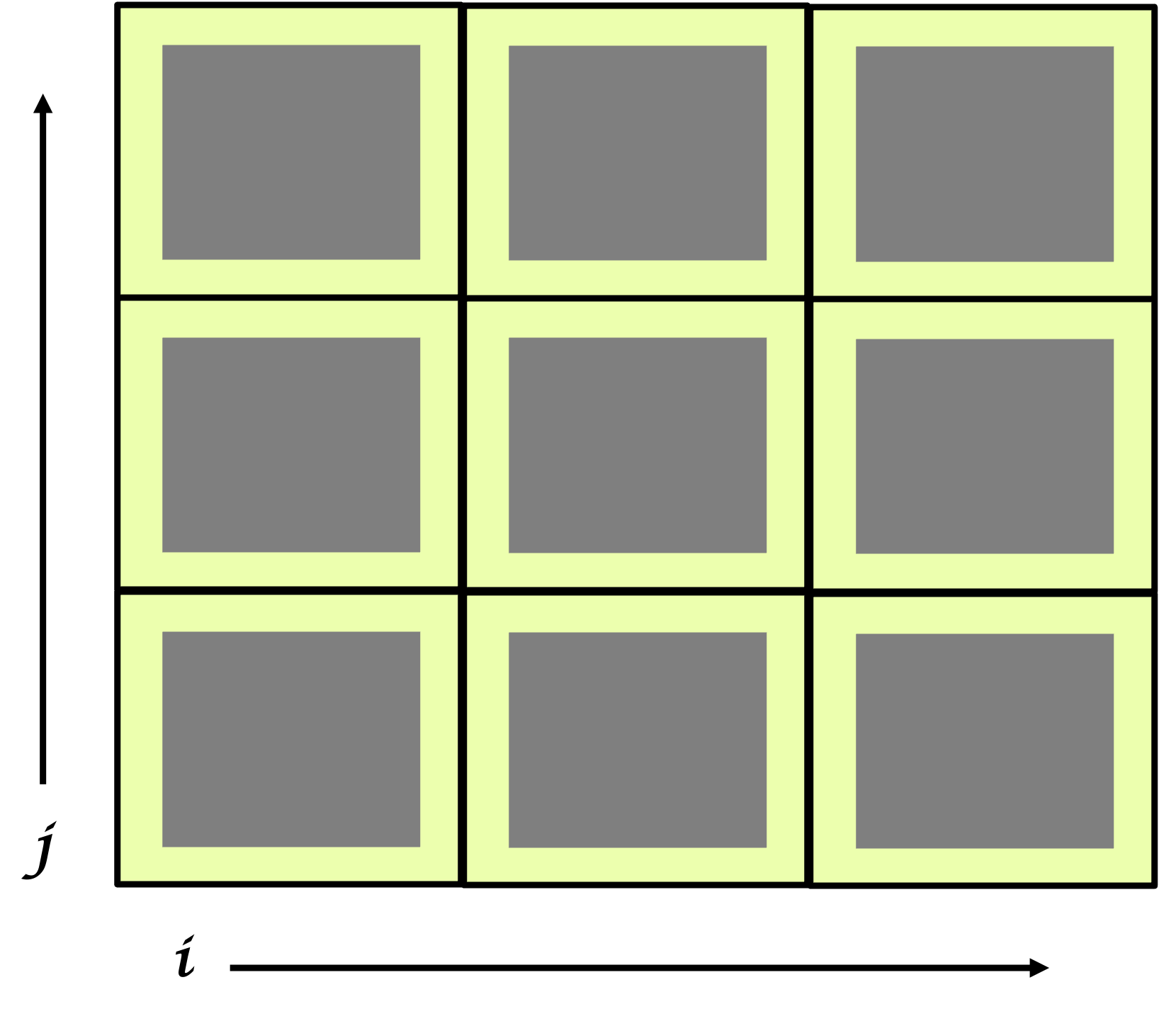
Distributed-memory parallelism takes place over patches, which are sections of the model domain allocated to a single distributed memory node. These patches send and receive information from each other (message passing). WRF uses HALO regions to assist with this. The image below shows an imaginary domain that is using nine processors. Each of the nine squares represents a single patch and is computed by a single processor. The yellow (or lighter) surrounding area in each square is the halo region. Halos are able to communicate with halos in neighboring, tangential patches, sending and receiving information.

"An image that shows a domain divided into nine grid spaces (3x3). Each grid represents a patch that is processed by a single processing unit. Each patch has a thin outlined area that represents the halo region."

Shared-memory Communications
Shared-memory parallelism uses OpenMP and takes place over tiles within patches. Tiles are sections of a patch allocated to a shared-memory processor within a single node. With shared memory processing, the domain is split among the run-time available OpenMP threads, and this is not sufficient for larger jobs (use dmpar instead for those). OpenMP is always within a single shared-memory processing unit.

Quilting¶

Note

This option is unstable and may not work properly.
This option is only used for wrf.exe. It does not work for real or ndown.

This option allows reserving a few processors to manage output only, which can be useful and performance-friendly if the domain size is large, and/or the time taken to write an output time is significant when compared to the time taken to integrate the model in between output times. There are two variables for setting the options:

nio_tasks_per_group: Number of processors to use per I/O group for I/O quilting (1 or 2 is typically sufficient)
nio_groups: How many I/O groups for I/O (default is 1).

Software Documentation¶

Detailed and comprehensive documentation aimed at WRF software is available in WRF v2 Software Tools and Documentation. Though the document was written for WRFv2, the information is still relevant for current versions.

Performance¶

Benchmark information for some WRF model versions is available from the WRF Benchmarks page.