WRF Physics

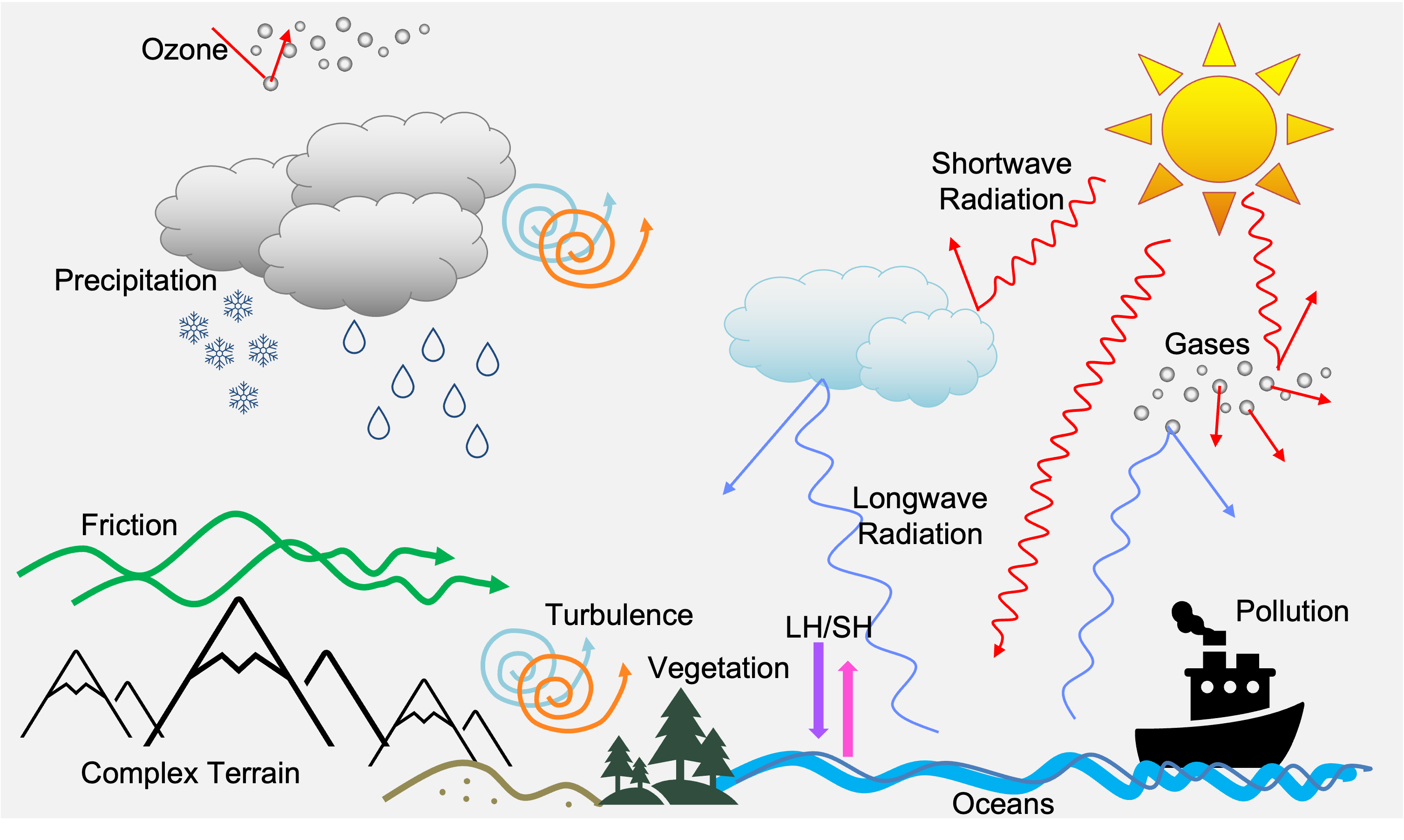
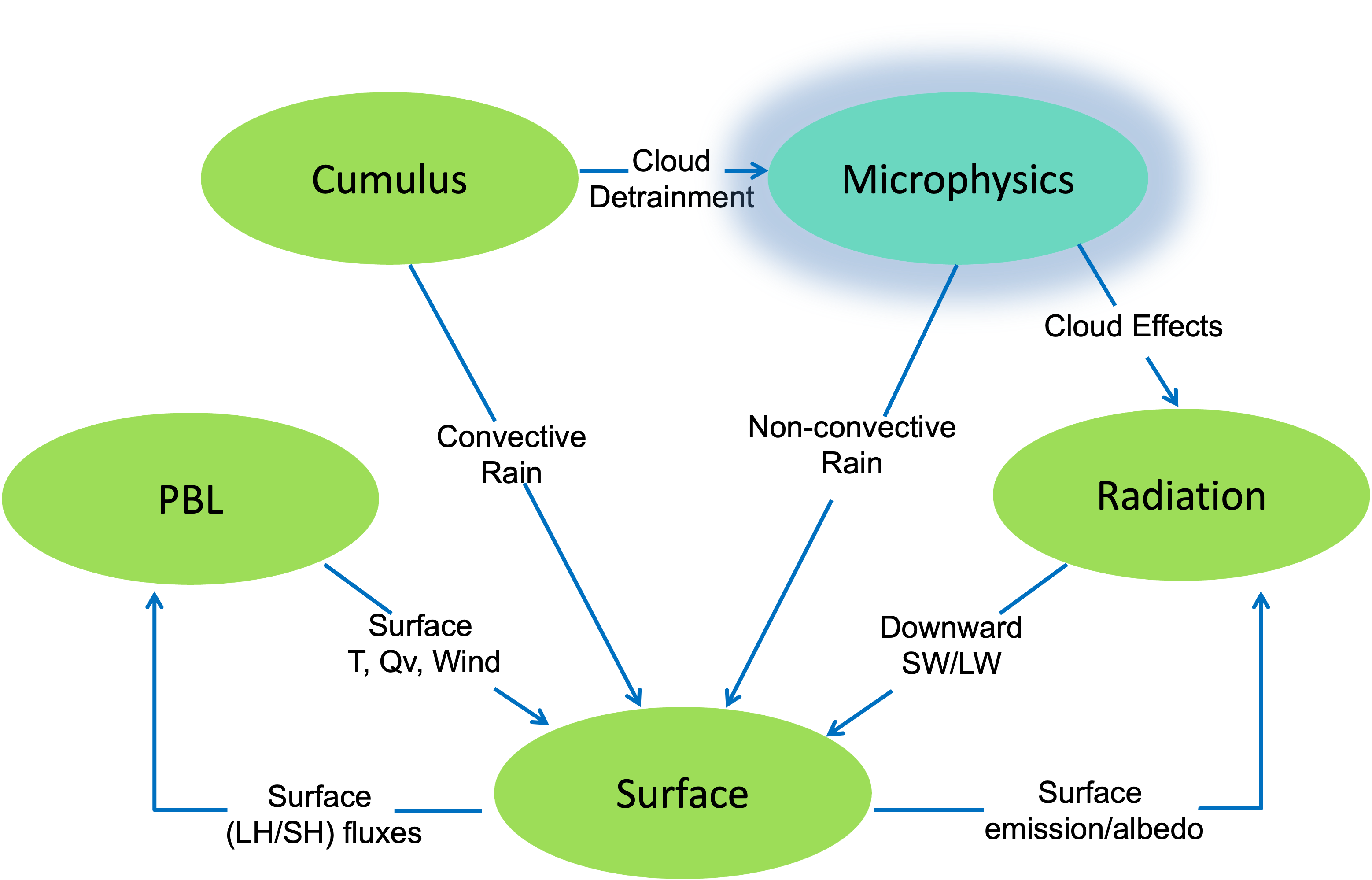
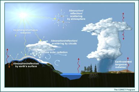
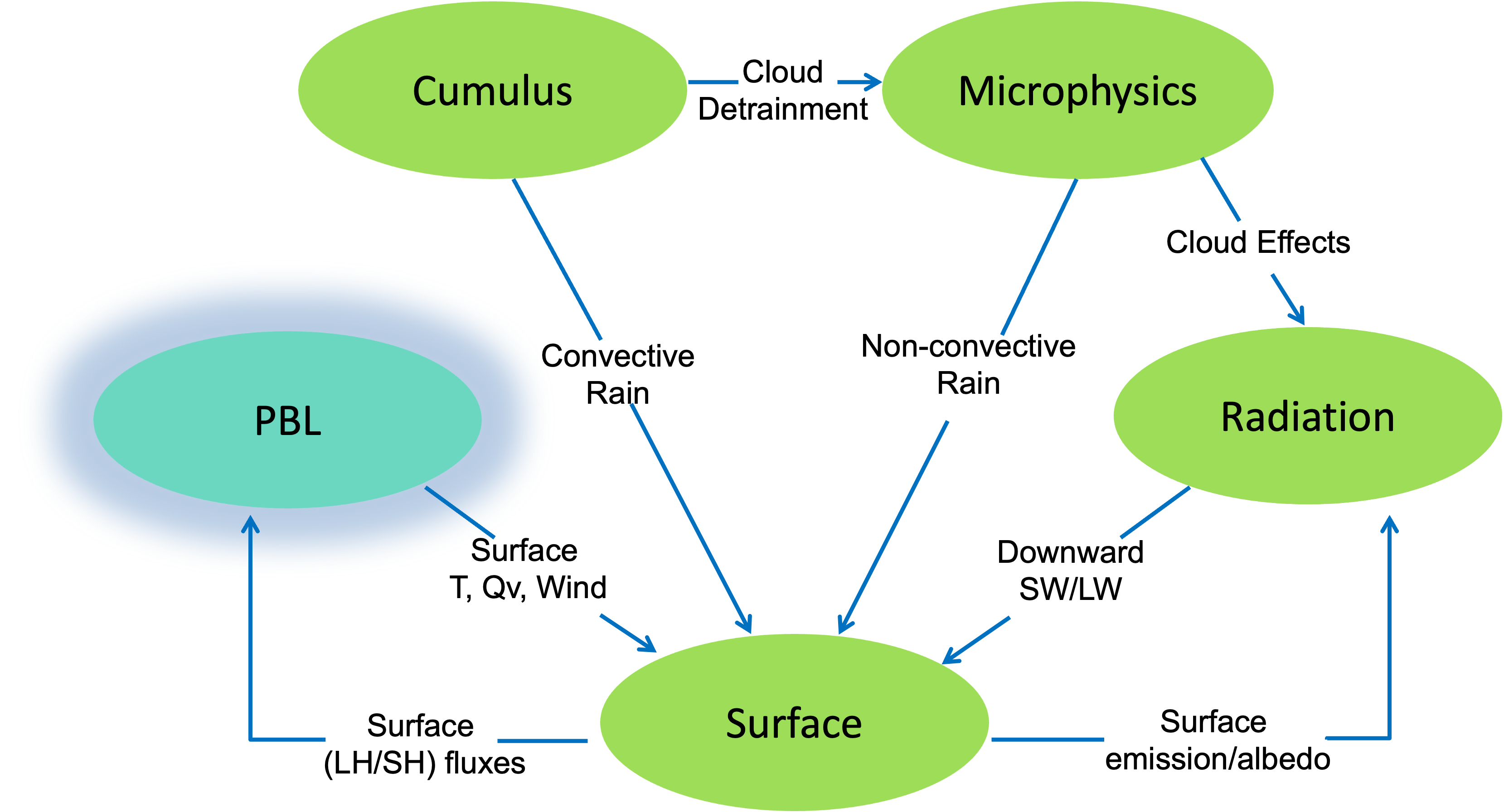
Earth’s atmosphere houses a variety of interacting physical processes, as are illustrated in the above image.

• Shortwave radiation from the sun is absorbed, reflected, and/or scattered by Earth’s surface, clouds, aerosols, gases, etc.

• Longwave radiation emitted from Earth’s surface either exits the atmosphere or is deflected back by gas particles and clouds.

• Heating from diurnal radiation creates a boundary-layer, which increases turbulence and potentially convection.

• Clouds are created by radiative or lifting processes, and produce precipitation in various forms (e.g., rain, snow, and graupel).

• Chemical components (e.g., aerosols, ozone, and pollutants) can modify clouds and radiation.

• At the surface, the roughness and other properties of land types (e.g., mountains, trees, buildings) modify surface fluxes.

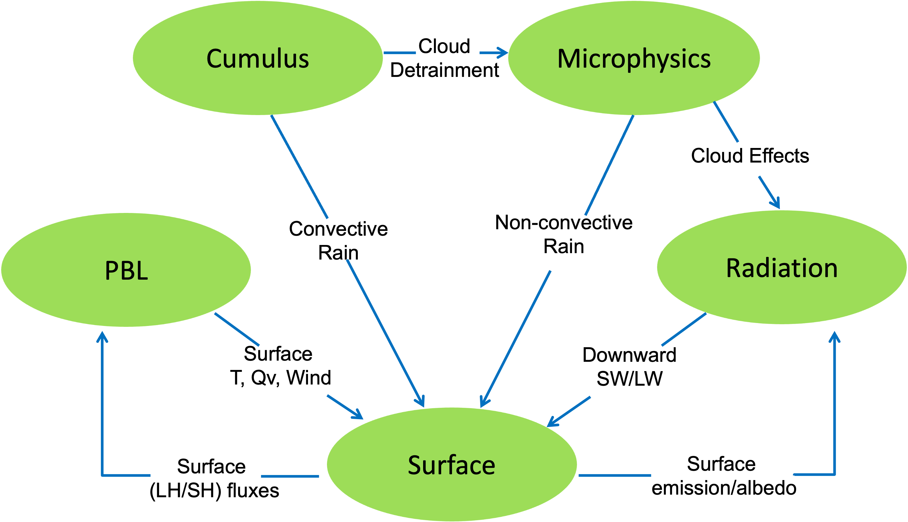
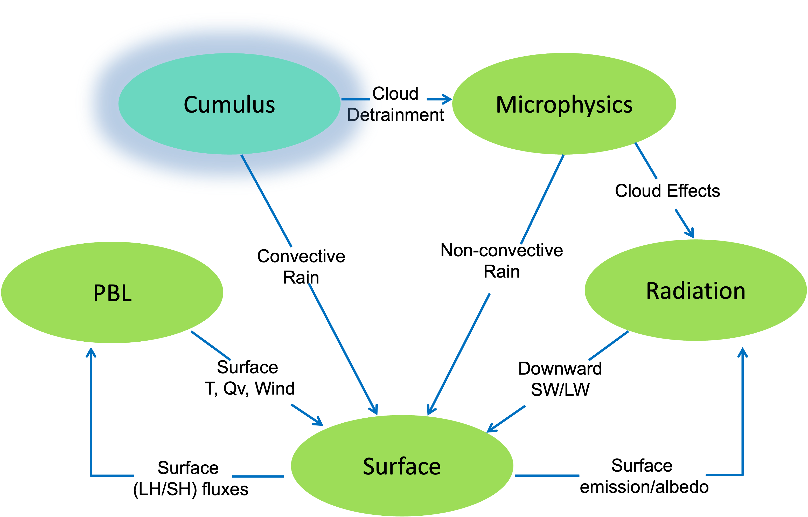
All of these processes work together to create our weather and climate. The WRF model code offers various physics that employ different calulation methods to best represent Earth’s atmospheric. The below image illustrates the ways in which the schemes interact.

Cumulus Parameterization

WRF Cumulus Parameterization Schemes

Physics schemes that parameterize sub-grid-scale effects of convective and shallow clouds.

Cumulus schemes activate column-by-column, depending on the presence of convective instability, and are responsible for the following:

• Providing column tendencies of heat and moisture to the model

• Providing the convective component of surface rainfall to the model

• Redistributing air in gridded columns to account for vertical convective fluxes

  • Updrafts lift boundary layer air, while downdrafts bring mid-level air downward. Schemes determine when and how quickly to trigger a convective column.

WRF cumulus schemes (except BMJ) are mass flux schemes, determining updraft/downdraft mass (and other) fluxes - this can include momentum transport. Updrafts, driven by buoyancy, send moist surface air up to the upper troposphere, and condensation becomes convective rainfall. Downdrafts occur when convective rain evaporates, which cools air to the boundary layer. Subsidence, the primary warming contributor in the column, warms and dries the troposphere. The BMJ scheme is an adjustment type, and relaxes toward a post-convective (mixed) sounding.

It is not always necessary to use cumulus parameterization. It is designed for grid sizes unable to parameterize the convective processes (i.e., when updrafts and downdrafts are sub-grid).

The following are general rules for WRF cumulus parameterization, which are illustrated in the above image:

Domain Grid Spacing	Guidelines
>=10km	a cumulus scheme is necessary
<=3km	a cumulus scheme is likely unnecessary, though it may help if convection exists just prior to the simulation start time
>=3km to <=10km	This is a “gray zone” where cumulus parameterization may or may not be necessary; try to avoid domains this size; if unavoidable, use the Multi-scale Kain Fritsch or Grell-Freitas scheme, which account for these scales.

See also

See the WRF Tutorial presentation on cumulus parameterization for additional details.

Cumulus Options

Moisture tendencies below represent mixing ratios of:

• c : cloud water

• r : rain water

• i : cloud ice

• s : snow

Scheme	Option	Moisture Tendencies	Momentum Tendencies	Shallow Convection	Radiation Interaction
Kain-Fritsch (KF)	1	Qc Qr Qi Qs	no	yes	yes
BMJ	2	N/A	no	yes	GFDL
Grell-Freitas	3	Qc Qi	no	yes	yes
Old SAS	4	Qc Qi	no	yes	GFDL
Grell-3	5	Qc Qi	no	yes	yes
Tiedtke	6	Qc Qi	yes	yes	no
Zhang-McFarlane	7	Qc Qi	yes	yes	RRTMG
KF-CuP	10	Qc Qi	no	yes	yes
Multi-scale KF	11	Qc Qr Qi Qs	no	yes	?
KIAPS SAS	14	Qc Qi	yes	use shcu_physics=4	GFDL
New Tiedtke	16	Qc Qi	yes	yes	no
Grell-Devenyi	93	Qc Qi	no	no	yes
NSAS	96	Qc Qi	yes	no/yes	GFDL
Old KF	99	Qc Qr Qi Qs	no	no	GFDL

Cumulus Details and References

Kain-Fritsch (KF)

cu_physics=1
Deep and shallow convection sub-grid scheme using a mass flux approach with downdrafts and CAPE removal time scale
Kain, 2004

The following additional options may be used with this scheme:

• kfeta_trigger :

  • =1 : default trigger

  • =2 : moisture-advection modulated trigger function (Ma and Tan, 2009), which can improve results in subtropical regions with weak large-scale forcing

  • =3 : RH-dependent perturbation - additional to option 1

  
  

• cu_rad_feedback=.true. : allows sub-grid cloud fraction interaction with radiation (Alapaty et al., 2012)

Betts-Miller-Janjic (BMJ)

cu_physics=2
Operational Eta scheme. Column moist adjustment scheme relaxing towards a well-mixed profile.
Janjic, 1994

Grell-Freitas (GF)

cu_physics=3
An improved Grell-Devenyi (GD) that attempts smoothing the transition to cloud-resolving scales, as proposed by Arakawa et al., 2004
Grell and Freitas, 2014

Simplified Arakawa-Schubert (SAS)

cu_physics=4
Simple mass-flux scheme with quasi-equilibrium closure, that includes a shallow mixing scheme.
Pan et al., 1995

Grell 3D (G3)

cu_physics=5
An improved Grell-Devenyi (GD) that can be used with high (and coarse) resolution when subsidence spreading (cugd_avedx) is turned on.
Grell, 1993
Grell and Devenyi, 2002

Tiedtke scheme

cu_physics=6
(U. of Hawaii version); Mass-flux scheme with a CAPE-removal time scale, shallow component, and momentum transport.
Tiedtke, 1989
Zhang et al., 2011

Zhang-McFarlane

cu_physics=7
Mass-flux CAPE-removal deep convection scheme with momentum transport - from the CESM climate model.
Zhang and McFarlane, 1995

Kain-Fritsch (KF)

cu_physics=10
Cumulus Potential scheme, which modifies the KF ad-hoc trigger function. This scheme links to boundary layer turbulence via probability density functions (PDFs) and computes cumulus cloud fraction based on a time scale relevant for shallow cumuli.
Berg et al., 2013

Multi-scale Kain-Fritsch

cu_physics=11
LCC-based entrainment, using a scale-dependent dynamic adjustment timescale and a trigger function based on Bechtold et al., 2001; includes an option to use CESM aerosol. Since wrfv4.2 convective momentum transport is added and turned on, by default - turn off by setting cmt_opt_flag = .false. in wrf/phys/module_cu_mskf.F - then recompile WRF (no need to use ‘clean -a’ or reconfigure).
Zheng et al., 2016
Glotfelty et al., 2019

KIAPS SAS (KSAS)

cu_physics=14
Based on New Simplified Arakawa-Schubert (NSAS), but scale-aware
Han and Pan, 2011
Kwon and Hong, 2017

New Tiedtke

cu_physics=16
Similar to the Tiedtke scheme used in REGCM4 and ECMWF cy40r1.
Zhang and Wang, 2017

Grell-Devenyi (GD)

cu_physics=93
A multi-closure, multi-parameter, ensemble method with (typically) 144 sub-grid members.
Grell and Devenyi, 2002

New Simplified Arakawa-Schubert (NSAS)

cu_physics=96
A mass-flux scheme with deep/shallow components, and momentum transport.
Han and Pan, 2011

Old Kain-Fritsch

cu_physics=99
Deep convection scheme that uses a mass flux approach, including downdrafts and a CAPE removal time scale.
Kain and Fritsch, 1990

Shallow Convection

In addition to cumulus parameterization, shallow convection schemes can be used for grid sizes in which shallow cumulus clouds (>1 km) are not resolved. These scheme allow non-precipitating shallow mixing to dry the planetary boundary layer, and then moisten and cool above by enhanced mixing, or with a mass-flux approach.

The following cumulus schemes already include shallow convection:

• Kain-Fritsch

• Old SAS

• KIAPS SAS

• Grell-3

• Grell-Freitas

• BMJ

• Tiedtke

The following standalone shallow schemes are available:

ishallow=1	Shallow convection that works with the Grell 3D scheme (cu_physics=5)
shcu_physics=2	UW (Bretherton and Park) shallow cumulus option from the CESM climate model - includes momentum transport Park et al., 2009
shcu_physics=3	GRIMS (Global/Regional Integrated Modeling System) scheme; represents the shallow convection process with eddy-diffusion and the pal algorithm, and couples directly to the YSU PBL scheme Hong and Jang, 2018
shcu_physics=4	NSAS shallow scheme; extracted from NSAS, and should be used with the KSAS deep cumulus scheme
shcu_physics=5	Deng shallow scheme; only works with the MYNN and MYJ PBL schemes; (available since wrfv4.1) Deng et al., 2003

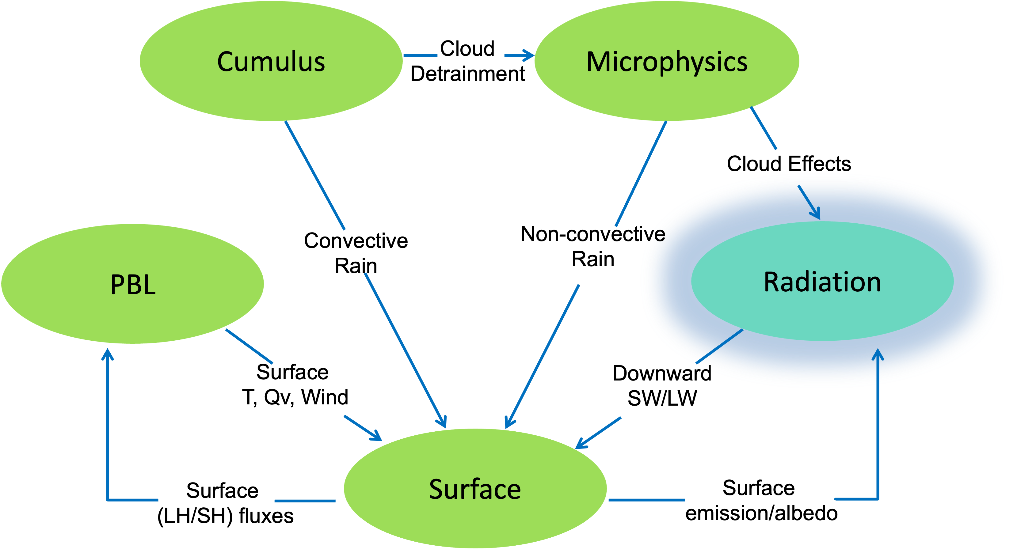
Microphysics

WRF Microphysics Schemes

Physics schemes that resolve cloud and precipitation processes, with some accounting for ice and/or mixed-phases processes.

WRF microphysics schemes provide atmospheric heat and moisture tendencies, and the resolved-scale (non-convective) rainfall at the surface. They consider various microphysical processes and different particle formation, depending on their type:

• Cloud droplets (10s of microns) condense from vapor at water saturation

• Rain (~mm diameter) forms from cloud droplet growth

• Ice crystals (10s of microns) form from droplet freezing or deposition on nuclei, which are assumed or explicit (e.g., dust particles)

• Snow (100s of microns) forms from growth of ice crystals at ice supersaturation and aggregation

• Graupel/hail (mm to cm) form and grow from mixed-phase interactions between water and ice particles

• Precipitating particles are typically assigned to an observationally-based size distribution

WRF includes the following types of microphysics schemes:

Note

More advanced scheme types are more computationally expensive.

Single-moment	Use a single prediction mass equation per species, where particle size distribution is derived from fixed parameters (Qr, Qs, etc.)
Double-moment	Add a number concentration prediction equation per double-moment species (Nr, Ns, etc.), allowing for additional processes (e.g., size-sorting during fall-out, aerosol effects, etc.)
Spectral bin	resolve size distribution by doubling mass bins

See also

See the WRF Tutorial presentation on microphysics for additional details.

Microphysics Options

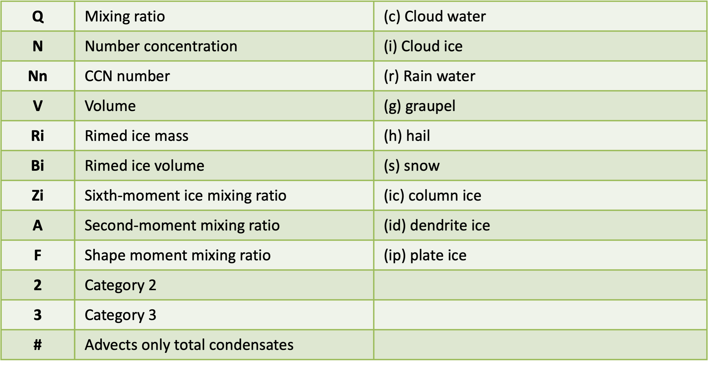
In the table below, abbreviations are defined as follows:

Scheme	Option	Mass Variables	Number Variables
Kessler	1	Qc Qr	N/A
Purdue Lin	2	Qc Qr Qi Qs Qg	N/A
WSM3	3	Qc Qr	N/A
WSM5	4	Qc Qr Qi Qs	N/A
Eta (Ferrier)	5	Qc Qr Qs Qt*	N/A
WSM6	6	Qc Qr Qi Qs Qg	N/A
Goddard 4-ice	7	Qc Qr Qi Qs Qg Qh	N/A
Thompson	8	Qc Qr Qi Qs Qg	Ni Nr
Milbrandt 2-mom	9	Qc Qr Qi Qs Qg Qh	Nc Nr Ni Ns Ng Nh
Morrison 2-mom	10	Qc Qr Qi Qs Qg	Nr Ni Ns Ng
CAM 5.1	11	Qc Qr Qi Qs	Nc Nr Ni Ns
SBU-YLin	13	Qc Qr Qi Qs	N/A
WDM5	14	Qc Qr Qi Qs	Nn Nc Nr
WDM6	16	Qc Qr Qi Qs Qg	Nn Nc Nr
NSSL	18	Qc Qr Qi Qs Qg Qh	Nc Nr Ni Ns Ng Nh Nn
WSM7	24	Qc Qr Qi Qs Qg Qh	N/A
WDM7	26	Qc Qr Qi Qs Qg Qh	Nc Nr
Thompson Aerosol	28	Qc Qr Qi Qs Qg	Nc Ni Nr Nn Nni
HUJI Fast	30	Qc Qr Qi Qs Qg	Nn Nc Nr Ni Ns Ng
Thompson Hail/Graupel/Aerosol	38	Qc Qr Qi Qs Qg	Nc Ni Nr Nn Nni Ng Vg
Morrison 2-mom Aerosol	40	Qc Qr Qi Qs Qg
P3	50	Qc Qr Qi	Nr Ni Ri Bi
P3-nc	51	Qc Qr Qi	Nc Nr Ni Ri Bi
P3-2nd	52	Qc Qr Qi2	Nc Nr Ni Ni2 Ri Ri2 Bi Bi2
P3-3mc	53	Qc Qr Qi	Nc Nr Ni Ri Bi Zi
ISHMAEL	55	Qc Qr Qi Qi2 Qi3	Nr Ni Ni2 Ni3 Vi Vi2 Vi3 Ai Ai2 Ai3
NTU	56	Qc Qr Qi Qs Qg Qh Qden Qten Qccn Qrcn	Nc Nr Ni Ns Ng Nh Nin Ai As Ag Ah Vi Vs Vg Fi Fs

Microphysics Option Details and References

Kessler

mp_physics=1
A warm-rain (no ice) scheme used commonly in idealized cloud modeling studies
Kessler, 1969

Purdue Lin

mp_physics=2
A sophisticated scheme that includes ice, snow, and graupel processes suitable for real-data high-resolution simulations
Chen and Sun, 2002

WRF Single-moment 3-class (WSM3)

mp_physics=3
A simple, efficient scheme with ice and snow processes, suitable for mesoscale grid sizes
Hong et al., 2004

WRF Single-moment 5-class (WSM5)

mp_physics=4
A slightly more sophisticated version of WRF Single-moment 3-class (WSM3) that allows for mixed-phase processes and super-cooled water
Hong et al., 2004

Ferrier Eta

mp_physics=5
The operational microphysics used in NCEP models; simple and efficient, with diagnostic mixed-phase processes; for fine resolutions (<5km)
NOAA, 2001

WRF Single-moment 6-class (WSM6)

mp_physics=6
Includes ice, snow and graupel processes, suitable for high-resolution simulations
Hong and Lim, 2006

Goddard 4-ice

mp_physics=7
Predicts hail and graupel separately; provides effective radii for radiation. Replaced older Goddard scheme since wrfv4.1.
Tao et al., 1989
Tao et al., 2016

Thompson et al.

mp_physics=8
Includes ice, snow and graupel processes suitable for high-resolution simulations
Thompson et al., 2008

Milbrandt-Yau Double-moment 7-class

mp_physics=9
Includes separate categories for hail and graupel with double-moment cloud, rain, ice, snow, graupel and hail
Milbrandt and Yau, 2005 (Part I)
Milbrandt and Yau, 2005 (Part II)

Morrison Double-moment

mp_physics=10
Double-moment ice, snow, rain and graupel for cloud-resolving simulations
Morrison et al., 2009

CAM V5.1 2-moment 5-class

mp_physics=11
User’s Guide to the CAM-5.1

Stony Brook University (Y. Lin)

mp_physics=13
A 5-class scheme with riming intensity predicted to account for mixed-phase processes
Lin and Colle, 2011

WRF Double-moment 5-class (WDM5)

mp_physics=14
Similar to WRF Single-moment 5-class (WSM5), but includes double-moment rain, and cloud and CCN for warm processes
Lim and Hong, 2010

WRF Double-moment 6-class (WDM6)

mp_physics=16
Similar to WRF Single-moment 6-class (WSM6), but includes double-moment rain, and cloud and CCN for warm processes
Lim and Hong, 2010

See also

• See WRF/doc/README.NSSLmp for details about NSSL microphysics schemes.

• If using WRF prior to v4.6.0, and an NSSL microphysics scheme, see NSSL Options Prior to v4.6.0.

NSSL 3-moment scheme with hail and CCN prediction

mp_physics=18
and either of the following:

• nssl_3moment=1 : predict radar reflectivity from rain

• nssl_3moment=2 : predict radar reflectivity of rain and hail

Mansell et al., 2010

Note

This option is available for WRF v4.6.0+.

NSSL 2-moment scheme with hail and CCN prediction

mp_physics=18
Mansell et al., 2010

NSSL 2-moment scheme without hail

mp_physics=18
and either of the following:

• nssl_hail_on=0

• nssl_ccn_on=0

Mansell et al., 2010

Note

This option is equivalent to mp_physics=22 from versions prior to v4.6.0.

NSSL 2-moment scheme with hail and constant background CCN

mp_physics=18, and
nssl_ccn_on=0
Mansell et al., 2010

Note

This option is equivalent to mp_physics=17 from versions prior to v4.6.0.

NSSL single-moment scheme, 7-class with predicted graupel density

mp_physics=18, and
nssl_2moment_on=0
nssl_ccn_on=0
Mansell et al., 2010

Note

This option is equivalent to mp_physics=19 from versions prior to v4.6.0.

NSSL single-moment scheme, 6-class with predicted graupel density

mp_physics=18, and
nssl_2moment_on=0
Mansell et al., 2010

Note

This option is equivalent to mp_physics=19 from versions prior to v4.6.0.

NSSL single-moment scheme, 6-class

mp_physics=18, and
nssl_2moment_on=0
nssl_hail_on=0
nssl_ccn_on=0
nssl_density_on=0
Mansell et al., 2010

Note

This option is equivalent to mp_physics=21 from versions prior to v4.6.0.

WRF Single-moment 7-class (WSM7)

mp_physics=24
Similar to WRF Single-moment 6-class (WSM6), but with an added hail category (effective beginning with v4.1)
Bae et al., 2018

WRF Double-moment 7-class (WDM7)

mp_physics=26
Similar to WRF Double-moment 6-class (WDM6), but with an added hail category (effective beginning with v4.1)
Bae et al., 2018

Thompson Aerosol-aware

mp_physics=28
Considers water- and ice-friendly aerosols
Thompson and Eidhammer, 2014

• A climatology data set may be used to specify initial and boundary conditions for the aerosol variables; includes a surface dust scheme.

• Since wrfv4.4 a black carbon aerosol category is added; biomass burning is an options.

Hebrew University of Jerusalem Fast (HUJI)

mp_physics=30
Spectral bin microphysics, fast version
Shpund et al., 2019

Thompson Hail/Graupel/Aerosol

mp_physics=38
Similar to Thompson Aerosol-aware, but computes two-moment prognostics for graupel and hail and includes a predicted density graupel category. Datafile qr_acr_qg_mp38V1.dat must be in the directory where wrf.exe is run, or it can alternatively be computed using namelist option write_thompson_mp38table=.true. (note this may take ~20 mins using 12 CPUs, ~5 mins with 128 CPUs, and several hours with a single CPU).

Morrison double-moment scheme with CESM aerosol

mp_physics=40
Similar to Morrison Double-moment, but with CESM aerosol added. This option is only valid with the Multi-scale Kain-Fritsch cumulus scheme (cu_physics=11) and requires CESM RCP4.5 data - after downloading, unpack the file and link one of the available files to the directory where wrf.exe is run.
No publication available for this specific scheme

Morrison and Milbrandt Predicted Particle Property (P3)

mp_physics=50
A single ice category representing a combination of ice, snow and graupel that carries prognostic arrays for rimed ice mass and volume; single-moment rain and ice.
Morrison and Milbrandt, 2015

Morrison and Milbrandt Predicted Particle Property (P3-nc)

mp_physics=51
As in Morrison and Milbrandt Predicted Particle Property (P3), but adds supersaturation-dependent activation and double-moment cloud water
Morrison and Milbrandt, 2015

Morrison and Milbrandt Predicted Particle Property (P3-2ice)

mp_physics=52
As in Morrison and Milbrandt Predicted Particle Property (P3), but with two ice arrays and double-moment cloud water
Morrison and Milbrandt, 2015

Morrison and Milbrandt Predicted Particle Property (P3-3moment)

mp_physics=53
As in Morrison and Milbrandt Predicted Particle Property (P3), but with 3-moment ice and double-moment cloud water
No publication available for this scheme

Jensen ISHMAEL

mp_physics=55
Predicts particle shapes and habits in ice crystal growth; (available since wrfv4.1)
Jensen et al., 2017

National Taiwan University (NTU)

mp_physics=56
Double-moment liquid phase and triple-moment ice phase, considers ice crystal shape and density variations; supersaturation is resolved so that condensation nuclei (CN) activation is explicitly calculated; CN’s droplet mass accounts for aerosol recycling.
Tsai and Chen, 2020

Radiation

WRF Radiation Schemes

WRF physics schemes that obtain cloud properties from the microphysics scheme to compute atmospheric temperature tendency profiles and longwave/shortwave surface radiative fluxes.

Longwave Radiation Schemes

Compute longwave radiation emitted and absorbed by the earth’s surface/clouds, and gases (e.g., water vapor, CO2). Wavelengths are thermal IR - longer than ~ 3 microns.

Shortwave schemes

Compute incoming solar fluxes reflected by Earth’s surface/clouds or absorbed by gases (e.g., water vapor, ozone, aerosols). These schemes account for annual and diurnal cycles and include ultraviolet, visible, and near-IR solar spectrum wavelengths.

See also

See the WRF Tutorial presentation on radiation for additional details.

Longwave Radiation Schemes

WRF longwave radiation schemes:

• Compute clear-sky and cloud upward and downward raditation fluxes

• Consider infrared emissions from layers

• Calculate surface emissivity based on the land type at each grid point

• Cools each layer, due to flux divergence of layer emissions

• Considers downward flux at the surface, which is crucial to the land-energy budget

• Infrared radiation generally leads to cooling in clear air (~2K/day), with stronger cooling at cloud tops and warming at cloud bases

In the table below, microphysics interactions represent mixing ratios of:

• c : cloud water

• r : rain water

• i : cloud ice

• s : snow

• g : graupel

Scheme	Option	Microphysics Interaction	Cloud Fraction	GHG
RRTM	1	Qc Qr Qi Qs Qg	1/0	constant or yearly GHG
CAM	3	Qc Qi Qs	Max-rand overlap	yearly CO2 or GHG
RRTMG	4	Qc Qr Qi Qs	Max-rand overlap	constant or yearly GHG
New Goddard	5	Qc Qr Qi Qs Qg	Max-rand	constant
FLG	7	Qc Qr Qi Qs Qg	1/0	constant
RRTMG-K	14	Qc Qr Qi Qs	Max-rand overlap	constant
Held-Suarez	31	none	none	none
GFDL	99	Qc Qr Qi Qs	Max-rand overlap	constant

The following are WRF’s available longwave radiation schemes:

RRTM

ra_lw_physics=1
Rapid Radiative Transfer Model. An accurate scheme using look-up tables for efficiency. Accounts for multiple bands, and microphysics species. For trace gases, the volume-mixing ratio values are CO2=379e-6, N2O=319e-9 and CH4=1774e-9. See the time-varying option in Options for Radiation Input.
Mlawer et al., 1997

CAM

ra_lw_physics=3
An option from CESM’s CAM 3 climate model that allows for aerosols and trace gases. It uses yearly CO2, and constant N2O (311e-9) and CH4 (1714e-9). See the time-varying option in Options for Radiation Input.
Collins et al., 2004

RRTMG

ra_lw_physics=4
A newer version of RRTM that includes the MCICA random cloud overlap method. For major trace gases, CO2=379e-6 (valid for 2005), N2O=319e-9, CH4=1774e-9. See the time-varying option in Options for Radiation Input.
Since wrfv4.2, the CO2 value is determined by the function: CO2(ppm) = 280 + 90 exp (0.02*(year-2000)). This function exhibits approximately 4% error when compared to observed values from the 1920s and 1960s, and about 1% error for years after 2000. A cloud overlap option is available beginning in wrfv4.4.
Iacono et al., 2008

New Goddard

ra_lw_physics=5
An efficient scheme with multiple bands that uses ozone from simple climatology. It is designed to run with Goddard microphysics particle radius information. The scheme had an update in wrfv4.1.
Chou and Suarez, 1999
Chou et al., 2001

Fu-Liou-Gu (FLG)

ra_lw_physics=7
A scheme with multiple bands that includes cloud and cloud fraction effects and profiles ozone based on climatology and tracer gases CO2=345e-6.
Gu et al., 2011
Fu and Liou, 1992

RRTMG-K

ra_lw_physics=14
An improved version of the RRTMG scheme.
Baek, 2017

Note

To use this option, WRF must be built with the configuration setting -DBUILD_RRTMK = 1 (this can be set by modifying configure.wrf prior to building WRF).

RRTMG-fast

ra_lw_physics=24
A fast version of the RRTMG scheme for GPUs and MIC. Beginning in wrv4.2, the following are the default GHG values:

• co2vmr=(280. + 90.*exp(0.02*(yr-2000)))*1.e-6

• n2ovmr=319.e-9

• ch4vmr=1774.e-9

• cfc11=0.251e-9

• cfc12=0.538e-9

Iacono et al., 2008

GFDL

ra_lw_physics=99
This is the Eta operational radiation scheme - an older multi-band scheme with carbon dioxide, ozone and microphysics effects
Fels and Schwarzkopf, 1981

Shortwave Radiation Schemes

WRF shortwave radiation schemes:

• Compute clear-sky and cloudy solar fluxes

• Include annual and diurnal solar cycles

• Consider downward and upward (reflected) fluxes (with the exception of the Dudhia (option 1) scheme, which only considers downward flux)

• Have a primarily warming effect in clear sky

• Are an important component of surface energy balance

In the table below, microphysics interactions represent mixing ratios of:

• c : cloud water

• r : rain water

• i : cloud ice

• s : snow

• g : graupel

Scheme	Option	Microphysics Interaction	Cloud Fraction	GHG
Dudhia	1	Qc Qr Qi Qs Qg	1/0	none
Goddard	2	Qc Qi	1/0	5 profiles
CAM	3	Qc Qi Qs	Max-rand overlap	lat/month
RRTMG	4	Qc Qr Qi Qs	Max-rand overlap	1 profile or lat/month
New Goddard	5	Qc Qr Qi Qs Qg	Max-rand	5 profiles
FLG	7	Qc Qr Qi Qs Qg	1/0	5 profiles
RRTMG-K	14	Qc Qr Qi Qs	Max-rand overlap	1 profile or lat/month
GFDL	99	Qc Qr Qi Qs	Max-rand overlap	lat/month

The following are WRF’s available shortwave radiation schemes:

Dudhia

ra_sw_physics=1
A scheme that uses simple downward integration, allowing for efficient clear-sky absorption and scattering for clouds.
Dudhia, 1989

Goddard

ra_sw_physics=2
A two-stream, multi-band scheme that uses cloud effects and climatological ozone
Chou and Suarez, 1994
Matsui et al., 2018

CAM

ra_sw_physics=3
A scheme that originates from CESM’s CAM 3 climate model - allows for aerosols and trace gases
Collins et al., 2004

RRTMG

ra_sw_physics=4
A scheme that uses the MCICA random cloud overlap method; for major trace gases, use CO2=379e-6 (valid for 2005), N2O=319e-9, CH4=1774e-9. See the time-varying option in Options for Radiation Input. Since wrfv4.2, the CO2 value is determined by the function: CO2(ppm) = 280 + 90 exp (0.02*(year-2000)). This function exhibits approximately 4% error when compared to observed values from the 1920s and 1960s, and about 1% error for years after 2000.

To use the cloud overlap option (available beginning in wrfv4.4), add cldovrlp = 1,2,3,4,or 5. For cldovrlp=4 or 5, use the decorrelation length option idcor=0 or 1. See Namelist Variables for details.

New Goddard

ra_sw_physics=5
An efficient scheme with multiple bands that uses climatological ozone. It is designed to run with Goddard microphysics particle radius information. The scheme was updated in WRFv4.1.
Chou and Suarez, 1999
Chou et al., 2001

Fu-Liou-Gu (FLG)

ra_sw_physics=7
A scheme with multiple bands, cloud and cloud fraction effects, and uses a climatological ozone profile. This scheme has the ability to allow for aerosols
Gu et al., 2011
Fu and Liou, 1992

RRTMG-K

ra_sw_physics=14
An improved version of the RRTMG scheme
Baek, 2017

Note

To use this option, WRF must be built with the configuration setting -DBUILD_RRTMK = 1 (this can be modified in configure.wrf prior to compiling).

RRTMG-fast

ra_sw_physics=24
A fast version of RRTMG
Iacono et al., 2008

Held-Suarez

ra_sw_physics=31
A temperature relaxation scheme designed for idealized tests only
No publication available

GFDL

ra_sw_physics=99
The Eta operational two-stream, multi-band scheme that includes cloud effects and climatological ozone
Fels and Schwarzkopf, 1981

Namelist Options Related to Shortwave Radiation

slope_rad=1	include slope and shading effects; modifies surface solar radiation flux according to terrain slope
topo_shading=1	allows for shadowing of neighboring grid cells; use only with with a grid size less than a few kilometers
swrad_scat	scattering turning parameter for use with ra_sw_physics=1; default value is 1, which is equivalent to 1.e-5 m2/kg; when greater than 1, scattering is increased
ra_sw_eclipse=1	eclipse effect on shortwave radiation; only works with ra_sw_physics options 1 (Dudhia), 2 (Goddard), 4 (RRTMG), and 5 (New Goddard). Eclipse data from 1950 – 2050 is provided in WRF/run/eclipse_besselian_elements.dat.
swint_opt=1	interpolation of shortwave radiation based on the solar zenith angle code between shortwave calls
swint_opt=2	activates the Fast All-sky Radiation Model for Solar applications (FARMS), which is a fast radiative transfer model that allows simulations of broadband solar radiation every model time step. The model uses lookup tables of cloud transmittances and reflectances by varying cloud optical thicknesses, cloud particle sizes, and solar zenith angles. See Xie et al., 2016 for details.

Options for Radiation Input

CAM Green House Gases

This option incorporates yearly green house gases from 1765 to 2500. Radiation schemes (ra_lw_physics)) CAM (option 3), RRTM (option 1), and RRTMG (option 4) work with this option. Set the following in namelist.input to turn it on:

&physics
ghg_input = 1
ra_lw_physics = 1, 3, or 4

The following files contain different scenarios and are available in the WRF/test/em_real and WRF/run directories:

• from IPCC AR5: CAMtr_volume_mixing_ratio.RCP4.5/RCP6/RCP8.5

• from IPCC AR4: CAMtr_volume_mixing_ratio.A1B/A2

• from IPCC AR6: CAMtr_volume_mixing_ratio.SSP119/SSP126/SSP245/SSP370/SSP585

• the default points to the CAMtr_volume_mixing_ratio.SSP245 file

Note

The ghg_input namelist option is not available in versions prior to WRFv4.4. If using an older version, to activate this option, the code must be configured with the -DCLWRFGHG macro (or set in configure.wrf) prior to compiling.

RRTMG Climatological Ozone

When using RRTMG radiation (ra_sw(lw)_physics=4), ozone data, adapted from CAM radiation (ra_lw(sw)_physics=3), incorporates latitudinal (2.82 degrees), height, and monthly variations - unlike the default height-only option. Set the following in namelist.input to use this option:

&physics
 o3input = 2
 ra_sw_physics = 4 (for each domain)
 ra_lw_physics = 4 (for each domain)

RRTMG Aerosol Options

aer_opt = 1

Aerosol data based on Tegen et al., 1997 are available for use with RRTMG radiation (ra_sw(lw)_physics=4). The data have spatial (5 degrees in longitude and 4 degrees in latitudes) and monthly variations, and include:

• organic carbon

• black carbon

• sulfate

• sea salt

• dust

• stratospheric aerosol (volcanic ash, which is zero)

Set the following in namelist.input to use this option:

&physics
 aer_opt = 1
 ra_sw_physics = 4  (for each domain)
 ra_lw_physics = 4   (for each domain)

aer_opt = 2

When using RRTMG radiation (ra_sw(lw)_physics=4), Aerosol Optical Depth (AOD) - either alone or with the Angstrom exponent, single scattering albedo, and cloud asymmetry can be provided as constant namelist values or as 2D input fields (via auxiliary input stream 15), with an option to specify aerosol type. To activate this option, set the following in namelist.input:

&physics
 aer_opt = 2
 ra_sw_physics = 4 or 5 (for each domain)
 ra_lw_physics = 4 or 5 (for each domain)

aer_opt = 3

When using RRTMG radiation (ra_sw(lw)_physics=4) and Thompson aerosol-aware microphysics (mp_physics=28), climatological water- and ice-friendly aerosols can be used. To activate this option, use the following namelist.input settings:

&physics
 aer_opt = 2
 ra_sw_physics = 4 or 5 (for each domain)
 ra_lw_physics = 4 or 5 (for each domain)
 mp_physic = 28 (for each domain)

RRTMG Effective Cloud water, Ice and Snow Radii

When using RRTMG radiation (ra_sw(lw)_physics=4), effective cloud water, ice, and snow radii data are available with the following namelist.input setting:

&physics
 use_mp_re = 1
 ra_sw_physics = 4 or 5 (for each domain)
 ra_lw_physics = 4 or 5 (for each domain)

These data originate from the following microphysics schemes:

• Thompson (mp_physics=8)

• WSM (mp_physics=3,4,6,24)

• WDM (mp_physics=14,16,26)

• Goddard 4-ice (mp_physics=7)

• NSSL (mp_physics=17,18,19,21,22)

• P3 (mp_physics=50-53)

Clouds and Cloud Fraction Options

Longwave Radiation and Clouds

Every radiation scheme interacts with model-resolved cloud fields, which allows ice and water clouds and precipitating species, with the following nuances:

• Some microphysics options pass their own particle sizes (cloud droplets, ice and snow) to RRTMG radiation.

• Other combinations only use mass information from microphysics schemes, and assume effective sizes in the radiation scheme.

• Rain and graupel effects are smaller than cloud and snow, and are not often explicitly considered.

Clouds have a significant effect on infrared radiation (IR) across all wavelengths. Considered “grey bodies,” they are nearly opaque to it.

Shortwave Radiation and Clouds

Considerations for shortwave radiation schemes are similar to those of longwave schemes (above). There are interactions with model-resolved clouds, and, in some cases, cumulus schemes. There are fraction and overlap assumptions, as well as cloud albedo reflection. Surface albedo reflection is based on the land-surface type and snow cover.

Cloud Fraction for Microphysics Clouds

• icloud=1 : Xu and Randall method; fraction is only < 1 for small cloud amounts, 0 for no resolved cloud

• icloud=2 : Simple 0 or 1 method with small resolved cloud threshold

• icloud=3 : Thompson option (RH dependent); 1 > Fraction > 0 for high RH and no resolved clouds

Cloud Fraction for Unresolved Convective Clouds

• cu_rad_feedback=.true. : only works for Kain Fritsch (cu_physics=1), Grell Freitas (cu_physics=3), Grell 3 (cu_physics=5), Grell-Devenyi (cu_physics=93) cumulus options.

• ZM separately provides cloud fraction to radiation

Radiation Time Step

The namelist parameter radt (in the &physics record) controls the radiation time step. Consider the following when setting radt.

• Radiation is too expensive to call every step

• Frequency should resolve cloud-cover changes with time

• radt should be set to about one minute per km grid size (of the innermost domain) (e.g., radt=10 for \(dx=10000\) - or 10 km).

• When using feedback=1, it is recommended to set radt to the same value for each domain.

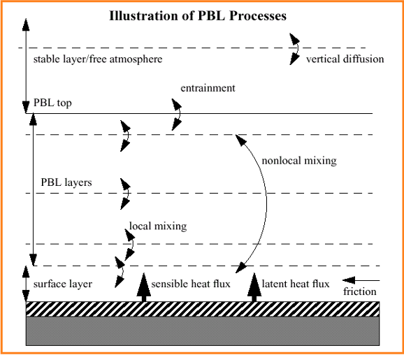
Planetary Boundary Layer Physics

WRF Planetary Boundary Layer (PBL) Schemes

WRF physics schemes that distribute surface fluxes with boundary layer eddy fluxes, allow for PBL growth by entrainment, and vertical mixing above the boundary layer.

There are two classes of PBL schemes:

1. Turbulent kinetic energy prediction schemes

   The following WRF PBL schemes fall under this class:

   • MYJ (bl_pbl_physics=2)

   • MYNN (bl_pbl_physics=5,6)

   • QNSE-EDMF (bl_pbl_physics=4)

   • BouLac (bl_pbl_physics=8)

   • CAM UW (bl_pbl_physics=9)

   • TEMF (bl_pbl_physics=10)

   
   

   QNSE-EDMF, MYNN, and TEMF schemes also include non-local mass-flux terms.

   
   

2. Diagnostic non-local schemes

   The following WRF PBL schemes fall under this class:

   • YSU (bl_pbl_physics=1)

   • GFS (bl_pbl_physics=3)

   • ACM2 (bl_pbl_physics=7)

   • MRF (bl_pbl_physics=99)

Note the following regarding WRF PBL schemes:

• Due to turbulence, all PBL schemes perform vertical diffusion above the PBL.

• PBL schemes can be used for most grid sizes when surface fluxes are present; however, this assumption breaks down at grid size \(dx << 1 km\), when 3-D diffusion should be used instead of a PBL scheme (coupled to surface physics). This works best when \(dx\) and \(dz\) are comparable.

• The lowest level should be located in the surface layer (0.1h) for correct surface (2m, 10m) diagnostic interpolation.

• With ACM2, GFS, and MRF PBL schemes, the lowest full level should be .99 or .995 (not too close to 1).

• TKE schemes and YSU can use thinner surface layers.

• PBL schemes assume PBL eddies are not resolved.

See also

See the WRF Tutorial presentation on PBLi for additional details.

PBL Scheme Options

Scheme	Option	Works With sfclay Option	Prognostic Variables	Diagnostic Variables	Cloud Mixing
YSU	1	1 91	none	exch_h	QC QI
MYJ	2	2	4	EL_PBL exch_h	QC QI
QNSE-EDMF	4	4	TKE_PBL	EL_PBL exch_h exch_m	QC QI
MYNN2	5	1 2 5 91	QKE	Tsq Qsq Cov exch_h exch_m	QC
MYNN3	6	1 2 5 91	QKE Tsq Qsq Cov	exch_h exch_m	QC
ACM2	7	1 7 91			QC QI
BouLac	8	1 2 91	TKE_PBL	EL_PBL exch_h exch_m	QC
UW	9	1 2 91	TKE_PBL	exch_h exch_m	QC
TEMF	10	10	TE_TEMF	*_temf	QC QI
Shin-Hong	11	1 91		exch_h	QC QI
GBM	12	1 91	TKE_PBL	EL_PBL exch_h exch_m	QC QI
EEPS	16	1 5 91	PEK_PBL PEP_PBL	exch_h exch_m	QC QI
KEPS	17	1 2	TPE_PBL DISS_PBL TKE_PBL	exch_h exch_m	QC
MRF	99	1 91			QC QI

PBL Scheme Details and References

Yonsei University (YSU)

bl_pbl_physics=1
A non-local-K scheme with an explicit entrainment layer and parabolic K profile in the unstable mixed layer. This option includes top-down mixing for turbulence, driven by cloud-top radiative cooling (this is separate from bottom-up surface-flux-driven mixing).
Hong et al., 2006

Additional options specific for use with YSU:

• topo_wind : =1 - applies a topographic correction to surface winds. The correction accounts for increased drag due to sub-grid topography and enhanced flow at hill tops (Jimenez and Dudhia, 2012); =2 - a simpler terrain variance-related correction

• ysu_topdown_pblmix=1 : applies top-down mixing driven by radiative cooling (Wilson and Fovell, 2018)

Mellor-Yamada-Janjic (MYJ)

bl_pbl_physics=2
Eta operational scheme - a one-dimensional prognostic turbulent kinetic energy scheme with local vertical mixing
Janjic, 1994
Mesinger, 1993

Quasi-Normal Scale Elimination (QNSE-EDMF)

bl_pbl_physics=4
A TKE-prediction option that incorporates a theory for stably-stratified regions. For the daytime, an eddy diffusivity mass-flux method with shallow convection (mfshconv=1) is used. It includes shallow convection using a mass-flux approach through the entire cloud-topped boundary layer
Sukoriansky et al., 2005

Mellor-Yamada Nakanishi and Niino Level 2.5 (MYNN2)

bl_pbl_physics=5
Predicts sub-grid TKE terms; includes shallow convection using a mass-flux approach through the entire cloud-topped boundary layer; includes top-down mixing for turbulence driven by cloud-top radiative cooling, which is separate from bottom-up surface-flux-driven mixing
Nakanishi and Niino, 2006
Nakanishi and Niino, 2009
Olson et al., 2019

Additional options specific for use with MYNN:

• icloud_bl=1 : option to couple MYNN subgrid-scale clouds with radiation

• bl_mynn_cloudpdf : =1 - Kuwano et al., 2010 ; =2 - Chaboureau and Bechtold, 2002 (with modifications; this is the default setting)

• bl_mynn_cloudmix=1 : mixing cloud water and ice (qnc and qni are mixed when scalar_pblmix=1)

• bl_mynn_edmf=1 : activate mass-flux in MYNN

• bl_mynn_mixlength : =1 is from RAP/HRRR; =2 is from blending

Mellor-Yamada Nakanishi and Niino Level 3 (MYNN3)

bl_pbl_physics=6
Predicts TKE and other second-moment terms
Nakanishi and Niino, 2006
Nakanishi and Niino, 2009
Olson et al., 2019

Note

This option is only available in versions, up through WRFv4.4.2. See the MYNN Closure option if using WRFv4.5+.

MYNN Closure

bl_mynn_closure

• = 2.5 : level 2.5

• = 2.6 : level 2.6

• = 3.0 : level 3.0

ACM2

bl_pbl_physics=7
Asymmetric Convective Model with non-local upward mixing and local downward mixing
Pleim, 2007

BouLac

bl_pbl_physics=8
Bougeault-Lacarrère PBL; a TKE-prediction option; for use with the BEP urban model (sf_urban_physics=2)
Bougeault, 1989

UW

bl_pbl_physics=9
A TKE scheme from the CESM climate model; includes shallow convection using a mass-flux approach from the cloud base; includes topdown mixing for turbulence driven by cloud-top radiative cooling, which is separate from bottom-up surface-flux-driven mixing
Bretherton and Park, 2009

Total Energy - Mass Flux (TEMF)

bl_pbl_physics=10
Sub-grid total energy prognostic variable, plus a mass-flux approach for shallow convection throughout the entire cloud-topped boundary layer
Angevine et al., 2010

Shin-Hong

bl_pbl_physics=11
Includes scale dependency for vertical transport in the convective PBL; vertical mixing in the stable PBL and free atmosphere follows Yonsei University (YSU); this scheme includes diagnosed TKE and mixing length output
Shin and Hong, 2015

Grenier-Bretherton-McCaa (GBM)

bl_pbl_physics=12
A TKE scheme that has been tested in cloud-topped PBL cases, and includes shallow convection using a mass-flux approach from the cloud base
Grenier and Bretherton, 2001

TKE (E)-TKE dissipation rate (epsilon) (EEPS)

bl_pbl_physics=16
This scheme predicts and advects both TKE and the TKE dissipation rate
No publication available

Note

This option only works with sf_sfclay_physics=1,5, or 91.

K-epsilon-theta² (KEPS)

bl_pbl_physics=17
This scheme includes two additional prognostic equations for dissipation rate and temperature variance.
Zonato et al., 2022

MRF

bl_pbl_physics=99
This is an older version of Yonsei University (YSU) (bl_pbl_physics=1) with implicit treatment of the entrainment layer as part of a non-local-K mixed layer
Hong and Pan, 1996

Additional PBL Options

LES PBL

Settings for a large-eddy-simulation (LES) boundary layer:

&physics
 bl_pbl_physic = 0 *(for each domain)*
 isfflx = 1
 sf_sfclay_physics = *any option, except 0* *(for each domain)*
 sf_surface_physics = *any option, except 0* *(for each domain)*
 diff_opt = 2  *(for each domain)*
 km_opt = 2 or 3  *(for each domain)*

• Diffusion is optional for vertical mixing.

• isfflx=0 or 2 can be used alternatively for idealized LES cases.

• Use \(dx \approx dz\), especially in the boundary layer, and avoid stretching to very large \(dz/dx\) aspect ratios at upper levels. This works better with continuous stretching to the top, instead of a fixed upper-level \(dz\) when \(dz >> dx\).

SMS-3DTKE

3D TKE subgrid mixing scheme that self-adapts to the grid size between the large-eddy simulation (LES) and mesoscale limits. This option is available with WRFv4.2+ and is activated with the following settings:

&physics
 bl_pbl_physic = 0  *(for each domain)*
 km_opt = 5  *(for each domain)*
 diff_opt = 2  *(for each domain)*
 sf_sfclay_physics = 1, 5, or 91 *(for each domain)*

See Zhang et al., 2018 for details.

Gravity Wave Drag

gwd_opt
An option to represent sub-grid orographic gravity-wave vertical momentum transport; can be used for all grid sizes with appropriate geogrid input fields

• =1 : (default); subgrid topography effects gravity wave drag and low-level flow blocking; recommended for all grid sizes; input wind is rotated to the Earth coordinate, and output is adjusted back to the projection domain, enabling use with all WRF-supported map projections; to apply this option, appropriate input fields from geogrid must be used; See Gravity Wave Drag Scheme Static Data for details.

  
  

• =3 : gravity wave drag, blocking, small-scale gravity drag and turbulent orographic form drag; similar to option 1, with the following additional subgrid-scale sources of orographic drag:

  1. Small-scale GWD (Tsiringakis et al., 2017), which represents gravity wave propagation and breaking in and above the stable boundary layer

  2. Turbulent orographic form drag (Beljaars et al., 2004)

  
  

  Both are applicable down to a grid size of 1 km. Large-scale GWD and low-level flow blocking from gwd_opt=1 are adjusted for horizontal grid resolution. More diagnostic fields from the scheme can be output by setting namelist option gwd_diags=1 in the &dynamics record. New GWD input fields are required from WPS.

Fog

grav_settling=2
Gravitational settling of fog/cloud droplets

PBL and Land Surface Time Step

The namelist parameter bldt (in the &physics record) controls the PBL time step in minutes between boundary layer and land-surface model calls. The default value of 0 (every step) is reasonable for all schemes, except the CLM land-surface scheme (sf_surface_physics = 5), which is expensive and bldt may need to be increased.

Model Grid Spacing

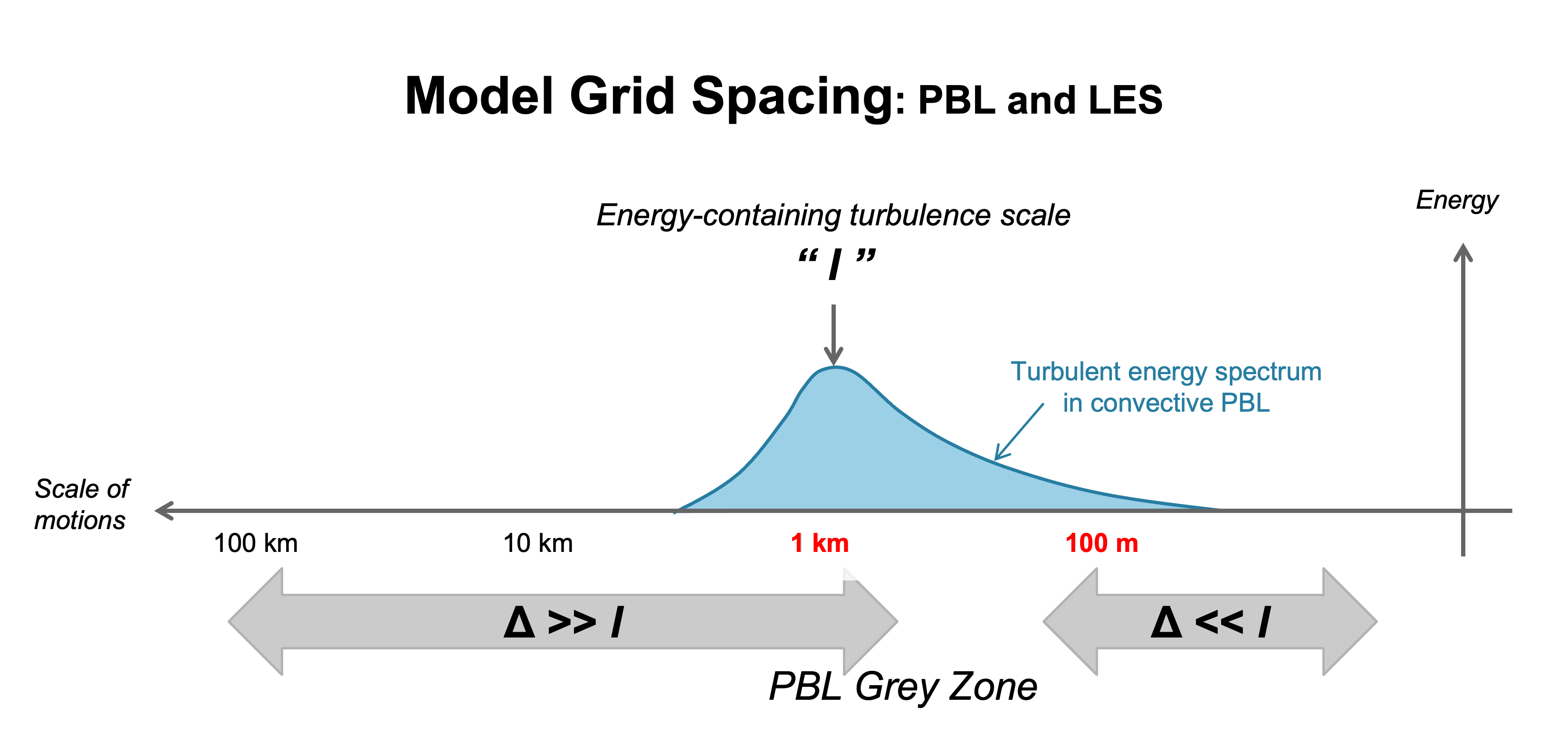
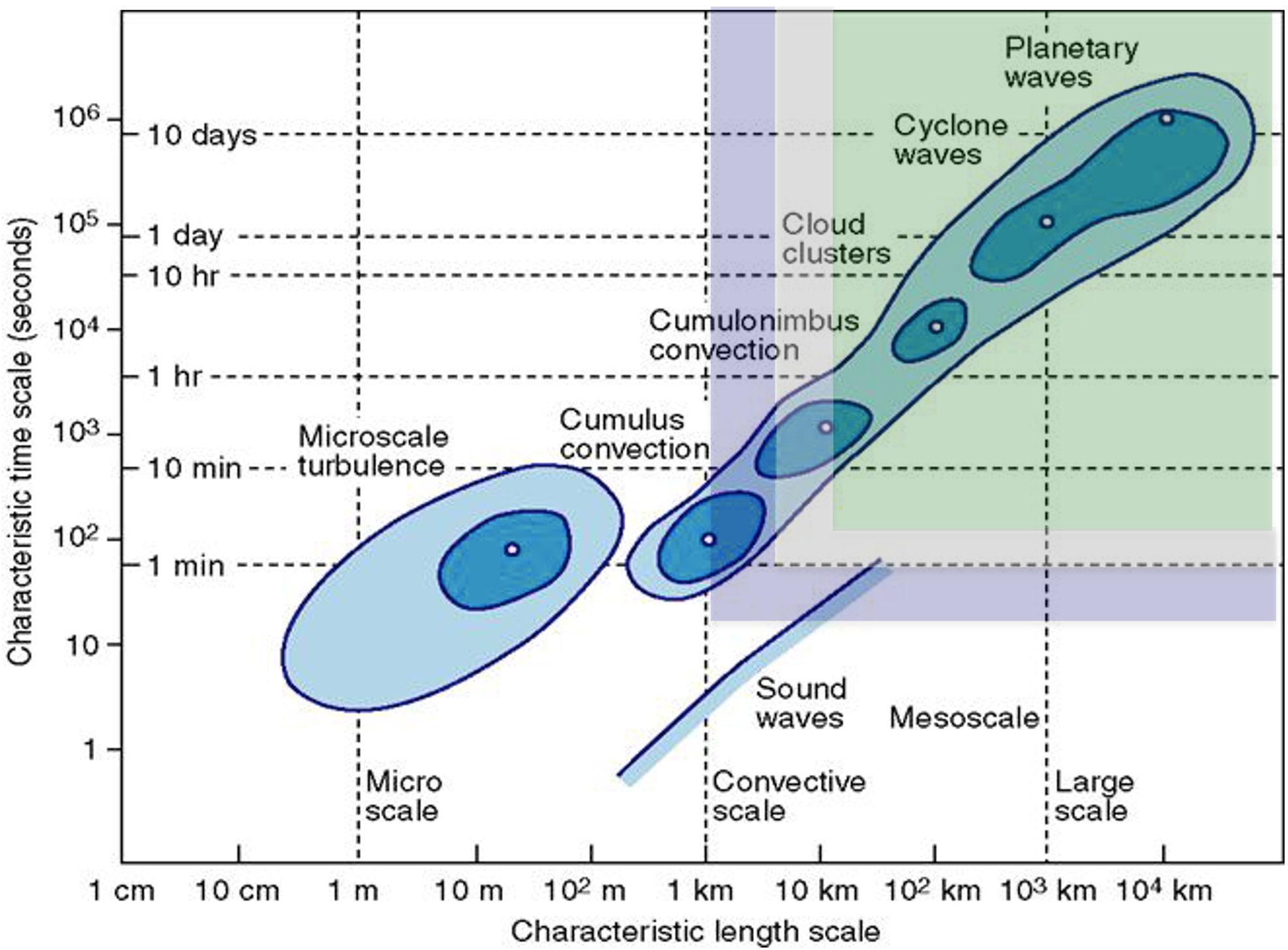
In the above image:

• WRF PBL schemes are designed for \(grid resolution >> I\)

• LES schemes are designed for \(grid resolution << I\)

With coarse grid spacing, eddies are sub-grid, and 1-D column schemes handle sub-grid vertical fluxes. For fine grid spacing, major eddies are resolved, and 3-D turbulence schemes handle sub-grid mixing.

The remaining sub-kilometer grid-spacing is a “grey-zone” with imperfect PBL and LES assumptions. The following scale-aware schemes are available for this zone:

• Shin-Hong PBL based on Yonsei University (YSU), designed for sub-kilometer transition scales (200 m – 1 km); nonlocal mass-flux; the \(Kv\) term is reduced in strength as grid size decreases and resolved mixing increases

• 3d TKE option (km_opt=5) (available in v4.2+); becomes 3-D LES at fine scales; adds scale-dependent Shin-Hong nonlocal mass flux and implicit vertical diffusion at coarse grid sizes

• Other schemes may work in this range but resolved/sub-grid energy fractions are not correctly partitioned.

LES is preferable for grid sizes up to about 100 m.

Turbulence and Diffusion

The diff_opt namelist option (in &dynamics) specifies the method used for turbulence and mixing. When diffusion is used with a PBL scheme, vertical diffusion is deactivated, therefore diff_opt only affects horizontal diffusion.

• diff_opt=0 : no turbulence or explicit spatial numerical filters

• diff_opt=1 : (default); evaluates the 2nd-order diffusion term on coordinate surfaces; uses the constant vertical diffusion coefficient (kvdif) unless a PBL option is used; do not use with calculated diffusion coefficient options (km_opt=2,3); can be used with PBL schemes that include internal vertical diffusion; horizontal diffusion acts along model levels - a simple numerical method with only neighboring points on the same model level

• diff_opt=2 : evaluates mixing terms in physical space (stress form - \(x,y,z\)); strictly horizontal and better for complex terrain - avoids diffusion up and down slopes included in diff_opt=1; horizontal diffusion acts strictly on horizontal gradients; the numerical method includes a vertical correction term, using more grid points; for stability, diffusion strength is reduced in steep coordinate slopes (\(dz \approx dx\))

Recommended Diffusion Options

1. Real-data case with PBL option on

   • diff_opt=2

   • km_opt=4

   • Less diffusive in complex terrain (while diff_opt=1 diffuses along slopes)

   • These options compliment the PBL scheme vertical diffusion

2. High-resolution real-data cases (~100m grid)

   • No PBL scheme

   • diff_opt=2

   • TKE (km_opt=2) or Smagorinsky scheme (km_opt=3)

3. Idealized cloud-resolving modeling (\(dx\) = 1-3 km ; smooth or no topography, no surface heat fluxes)

   • diff_opt=2

   • km_opt=2 or 3

Surface Physics

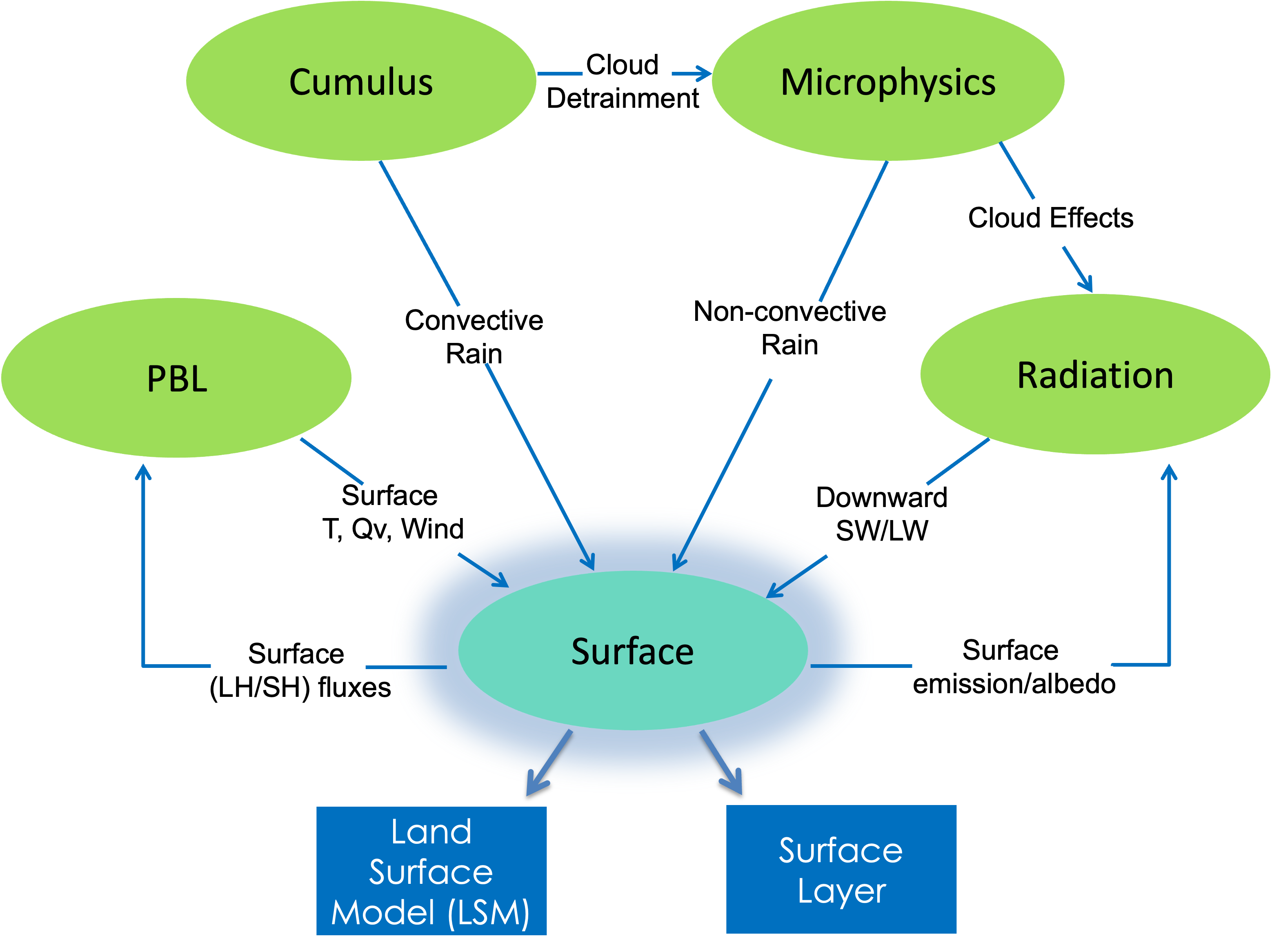
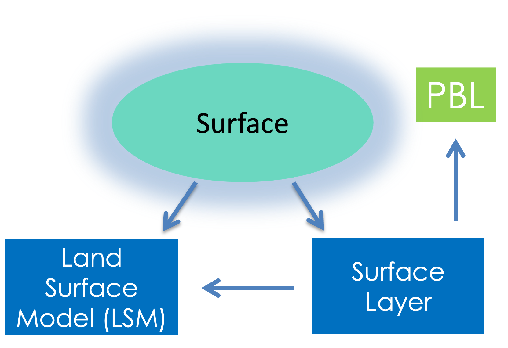
WRF surface physics consist of surface layer (sfclay) schemes and land surface model (LSM) schemes.

WRF Surface Layer (sfclay) Schemes

WRF physics schemes that determine surface layer diagnostics, including exchange and transfer coefficients, and determine soil temperature, moisture, snow prediction and sea-ice temperature. They provide heat and moisture exchange coefficients to the land surface model (LSM).

WRF Land Surface Model (LSM) Schemes

WRF physics schemes that provide land-surface fluxes of heat and moisture to the planetary boundary layer (PBL).

See also

See the WRF Tutorial presentation on surface physics for additional details.

Surface Layer Schemes

The surface layer has a constant flux layer of about 0.1 x PBL height (~100 m). The lowest WRF model level is found within this layer (typically 10-50 m).

The WRF surface layer scheme is determined by the namelist setting sf_sfclay_physics (in the &physics namelist record). Some key notes about WRF sfclay schemes are:

• They use similarity theory to determine exchange coefficients and diagnostics of 2m temperature, 2m qvapor, and 10m winds.

• They provide exchange coefficients to land-surface models (LSMs).

• They provide friction velocity to the PBL scheme.

• They provide surface fluxes over water points.

• Schemes have variations in stability functions and roughness lengths.

Surface Layer Scheme Details and References

Revised MM5

sf_sfclay_physics=1
Removes limits and uses updated stability functions; over the ocean, the COARE 3 forumula (Fairall et al., 2003) is used for thermal and moisture roughness lengths (or heat and moisture exchange coefficients)
Jimenez et al., 2012

Eta Similarity

sf_sfclay_physics=2
A scheme used in Eta model, based on Monin-Obukhov with Zilitinkevich thermal roughness length and standard similarity functions from look-up tables
Monin and Obukhov, 1954
Janjic, 1994
Janjic, 1996
Janjic, 2001

QNSE

sf_sfclay_physics=4
Quasi-Normal Scale Elimination PBL scheme’s surface layer option
No publication available

MYNN

sf_sfclay_physics=5
Nakanishi and Niino PBL’s surface layer scheme
Olson et al, 2021

Pleim-Xiu

sf_sfclay_physics=7
Pleim, 2006

Total Energy - Mass Flux (TEMF)

sf_sfclay_physics=10
Angevine et al., 2010

MM5 Similarity

sf_sfclay_physics=91
A scheme based on Monin-Obukhov, with Carslon-Boland viscous sub-layer and standard similarity functions from look-up tables; over the ocean, the COARE 3 forumula (Fairall et al., 2003) is used for thermal and moisture roughness lengths (or heat and moisture exchange coefficients)
Paulson, 1970
Dyer and Hicks, 1970
Webb, 1970
Belijaars, 1994
Zhang and Anthes, 1982

Additional Options Related to the Surface Layer

iz0tlnd

• =1 : Chen-Zhang thermal roughness length over land, which depends on vegetation height (works with sf_sfclay_physics = 1, 91, and 5)

• =0 : Original thermal roughness length in each sfclay option
  Chen and Zhang, 2009

shalwater_z0=1

Shallow-water roughness with an offshore roughness adjustment in water depths less tha 100 m. This option works with a specified depth or real bathymetry input, and only with sf_sfclay_physics=1. The bathymetry data is available from the WPS v4 Geographical Static Data Downloads Page. If no bathymetry data is available, set constant depth (in meters; must be positive) using namelist option shalwater_depth. Any depths outside the range of 10-100 m are rounded to the nearest limit value.
GEBCO Compilation Group, 2021
Jimenez and Dudhia, 2018

Land Surface Model

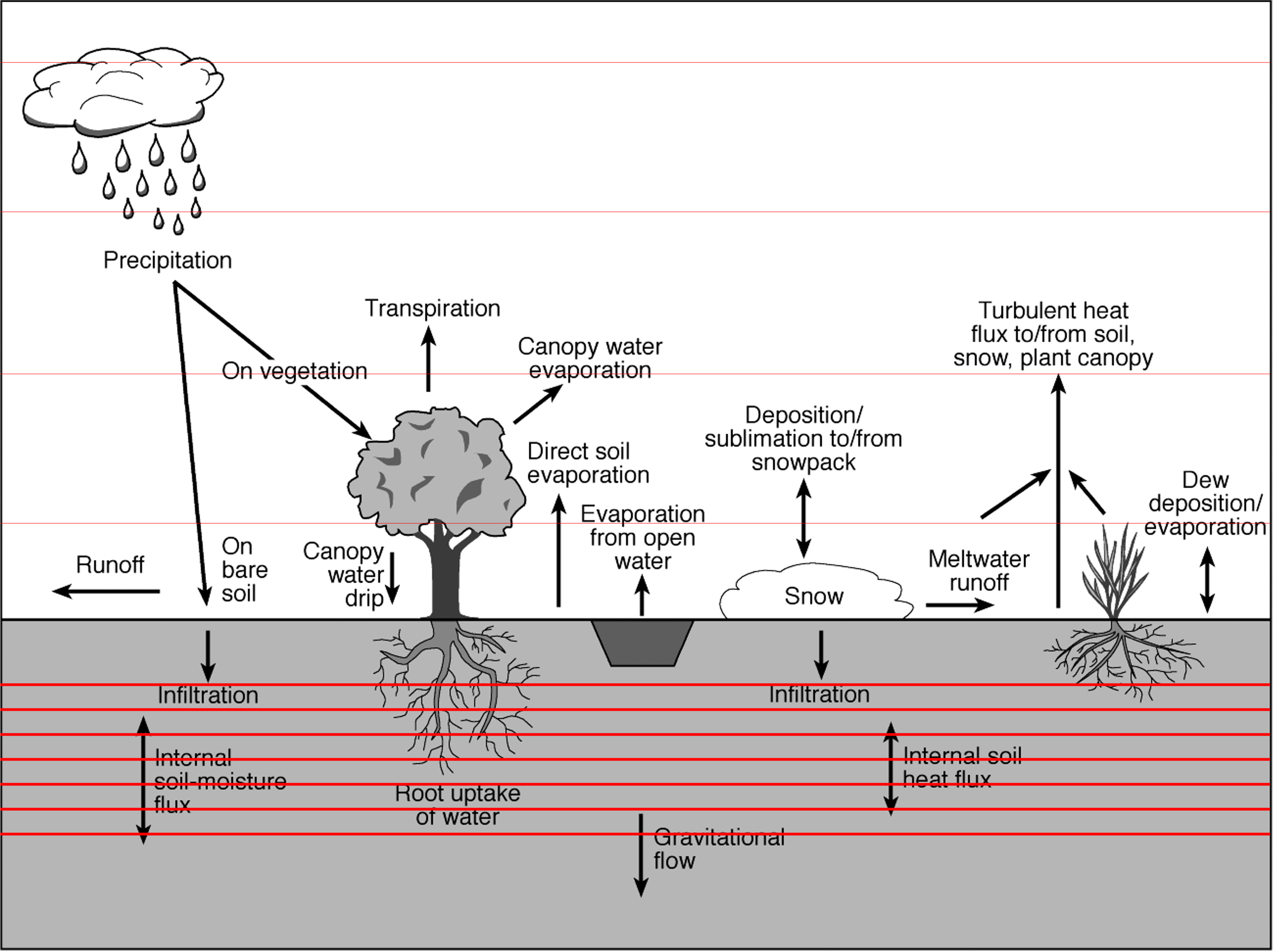
WRF LSM schemes are driven by surface energy and water fluxes. They predict soil temperature and soil moisture in 3 or 4 layers, depending on the scheme, as well as snow water equivalent on the ground.

Vegetation and Soil

LSMs consider the effects of vegetation and soil components, such as vegetation fraction, vegetation categories (e.g., cropland, forest types, etc.), and soil categories (e.g., sandy, clay, etc.). Below are some key notes:

• Processes include evapotranspiration, root zone, and leaf effects.

• Vegetation fraction varies seasonally.

• Soil categories are considered for drainage and thermal conductivity.

Snow Cover

LSMs include fractional snow cover and predict snow water equivalent development based on precipitation, sublimation, melting, and run-off. The number of layers is dependent on the scheme:

• Single-layer snow (Noah - sf_surface_physics=2, PX - sf_surface_physics=7)

• Multi-layer snow (RUC - sf_surface_physics=3, NoahMP - sf_surface_physics=4, CLM4 - sf_surface_physics=5, SSiB - sf_surface_physics=8)

• The 5-layer option - sf_surface_physics=2 - has no snow prediction

Note

Frozen soil water is also predicted by the Noah, NoahMP, RUC, and CLM4 schemes.

Urban Effects

For larger-scale studies, the LSM urban category is usually sufficient. Alternatively, urban models are available for use with either the Noah (sf_surface_physics=2) or NoahMP (sf_surface_physics=4) LSM scheme by setting sf_urban_physics in the &physics namelist record to one of the following options:

• =1 : Urban Canopy Model (UCM); single layer; The following options are available when sf_urban_physics=1

  • slucm_distributed_drag : An option to use spatially-varying 2-D urban zero-plane displacement, momentum roughness length, and frontal area index. This option requires SLUCM static input for the WPS/geogrid process

  • distributed_ahe_opt : An option to determine the method used for anthropogenic surface heat flux. An additional input to the wrfinput file is required.

    • =0 : do not use anthropogenic surface heat flux from the input data

    • =1 : (default) add to thefirst level temperature tendency

    • =2 : add to the surface sensible heat flux

  
  

• =2 : Building Environment Parameterization (BEP); multi-layer; only works with YSU, MYJ and BouLac PBL schemes (bl_pbl_physics= 1, 2, and 8)

• =3 : Building Energy Model (BEM); adds heating and air-conditioning to BEP; only works with YSU, MYJ and BouLac PBL schemes (bl_pbl_physics= 1, 2, and 8)

Note

• NUDAPT detailed map data is available for use in WPS, and includes data for 40+ U.S. cities.

• WRFv4.3+ code includes a capability to use local climate zones for all three urban applications (see the README file for details)

LSM Tables

LSM tables, found in WRF/test/em_real and WRF/run, are customizable text files with predefined categories.

Table	LSM scheme that uses the table
VEGPARM.TBL	Noah and RUC, for vegetation categories (albedo, roughness length, emissivity, vegetation properties)
MPTABLE.TBL	NoahMP
SOILPARM.TBL	Noah and RUC, for soil properties
LANDUSE.TBL	5-layer model (SLAB)
URBPARM.TBL	urban models

Initializing LSMs

All LSMs (except the SLAB option) require the following additional fields for initialization:

• Soil temperature

• Soil moisture

• Snow liquid equivalent

These fields are available in the first-guess input files processed in WPS. They originate from “offline” operational analysis or reanalysis modeling systems driven by observations for rainfall, radiation, surface temperature, humidity, and wind.

The following are model-derived data sets for Noah and RUC LSMs that correspond to WRF levels:

• Eta/GFS/AGRMET/NNRP for Noah (older data have limited soil levels)

• RUC for RUC (just North America; limited availability)

Note

When using ECMWF/ERA soil analyses, during real.exe mesoscale landuse resolution can cause inconsistency in elevation, soil type, and vegetation. Soil temperature adjustments occur during real.exe, and addresses elevation differences between the dataset and model elevations (using SOILHGT). Inconsistency leads to spin-up, as temperature and moisture adjustments occur at the beginning of simulation. This can be avoided by running an offline model on the same grid (e.g. HRLDAS for Noah), but soil moisture spin up may take months. Cycling the land state between forecasts also helps, but may propagate errors (e.g in rainfall effect on soil moisture).

LSM Scheme Details and References

5-layer thermal diffusion (SLAB)

sf_surface_physics = 1
A five-layer scheme that only considers soil temperature
Dudhia, 1996

Noah

sf_surface_physics = 2
The Unified NCEP/NCAR/AFWA four-layer scheme for soil temperature and moisture; includes fractional snow cover and frozen soil physics
Tewari et al., 2004

• Activate sub-tiling with sf_surface_mosaic=1 in the &physics namelist record. The mosaic_cat namelist option defines the number of tiles per grid box (default : 3).

RUC

sf_surface_physics = 3
This model calculates energy and moisture budgets using a layer approach. Atmospheric and soil fluxes, computed at the middle of the first atmospheric layer and the top soil layer respectively, modify heat and moisture storage in the ground surface layer. The RUC LSM utilizes 9 soil levels, with higher resolution near the atmosphere interface.

Note

Initializing from a low-resolution surface model, such as Noah LSM, can lead to overly moist top levels, causing moist/cold biases. The solution is to cycle soil moisture for several days, allowing it to spin up and align with the RUC LSM’s vertical structure.

The RUC LSM models soil moisture as a prognostic variable - volumetric soil moisture content, minus residual soil moisture, which does not contribute to transport. It incorporates soil freezing and thawing processes and can utilize explicit mixed-phase precipitation from cloud microphysics schemes. For sea ice, the model solves for heat diffusion, allowing for evolving snow cover. During the warm season, the RUC LSM adjusts soil moisture in cropland areas to account for irrigation.

On soil, snow accumulates in up to two layers, depending on its depth (ref S16). Thin layers combine with the topsoil layer to prevent excessive night time radiative cooling. If the snow water equivalent is below 3 cm, grid cells can be partially snow-covered, with surface parameters like roughness length and albedo calculated as a weighted average of snow-covered and snow-free areas.

The energy budget employs an iterative snow melting algorithm. Melted water may partially refreeze within the snow layer; the rest percolates through the snowpack, infiltrates the soil, forming surface runoff. Snow density evolves based on snow temperature, depth, and compaction. Snow albedo, initialized from the given vegetation type’s maximum albedo, can be adjusted according to snow temperature and snow fraction. To better represent accumulated snow on the ground, the RUC LSM includes an estimation of frozen precipitation density.

The RUC LSM includes refined interception of liquid or frozen precipitation by the canopy, and a “mosaic” approach for patchy snow, which separately treats energy and moisture budgets for snow-covered and snow-free portions of each grid cell, aggregating the solutions at the end of each time step.

The following data sets are required to initialize the RUC LSM:

• High-resolution soil and land-use types

• Climatological albedo for snow-free areas

• Spatial distribution of maximum surface albedo in the presence of snow cover

• Grid cell vegetation-type fraction - for sub-grid-scale heterogeneity in surface parameter computation

• Grid cell soil-type fraction

• Climatological greenness fraction

• Climatological leaf area index

• Climatological mean temperature at the bottom of soil domain

• Real-time sea-ice concentration

• Real-time snow cover to correct cycled-in RAP and HRRR snow fields

Recommended namelist options:

• sf_surface_physics=3

• num_soil_layers=9

• usemonalb=.true. ; uses monthly albedo fields from geogrid instead of table values

• rdlai2d=.true. ; uses monthly LAI data from geogrid, which is included in the wrflowinp file if sst_update=1

• mosaic_lu=1

• mosaic_soil=1

Note

See RAP and HRRR, which use RUC LSM as their land component.

Benjamin et al., 2004
Smirnova et al., 2016

Noah-MP

sf_surface_physics = 4
Uses multiple options for key land-atmosphere interaction processes, as well as the following:

• Contains a separate vegetation canopy, defined by its top and bottom, with leaf physical and radiometric properties utilized in a two-stream canopy radiation transfer scheme that accounts for shading effects

• Contains a multi-layer snow pack with liquid water storage, melt/refreeze capability, and a snow-interception model describing loading/unloading, melt/refreeze, and sublimation of the canopy-intercepted snow

• Multiple options are available for surface water infiltration and runoff, and groundwater transfer and storage, including water table depth to an unconfined aquifer

• Horizontal and vertical vegetation density can be prescribed or predicted using prognostic photosynthesis and dynamic vegetation models that allocate carbon to vegetation (leaf, stem, wood and root) and soil carbon pools (fast and slow)

Niu et al., 2011
Yang et al., 2011
Noah-MP Technical Note (He et al., 2023)

Community Land Model Version 4 (CLM4)

sf_surface_physics = 5
Contains sophisticated treatment of biogeophysics, hydrology, biogeochemistry, and dynamic vegetation. Each grid cell’s land surface is defined by five sub-grid land cover types: glacier, lake, wetland, urban, and vegetated. The vegetated sub-grid consists of up to 4 plant functional types (PFTs) that differ in physiology and structure. WRF input land cover types are translated into the CLM4 PFTs through a look-up table. The CLM4 vertical structure includes a single-layer vegetation canopy, a five-layer snowpack, and a ten-layer soil column.

Oleson et al., 2010
Lawrence et al., 2011

Note

An earlier version of CLM has been quantitatively evaluated within WRF; referenced in the following:
Jin and Wen, 2012
Lu and Kueppers, 2012
Subin et al., 2011

Pleim-Xiu

sf_surface_physics = 7
A two-layer scheme based on the ISBA model (Noilhan and Planton, 1989) that includes vegetation and sub-grid tiling, and provides realistic ground temperature, soil moisture, and surface sensible and latent heat fluxes in mesoscale models. It includes a 2-layer force-restore soil temperature and moisture model (1 cm thick top layer, 99 cm bottom layer). It derives grid aggregate vegetation and soil parameters from fractional coverage of land use categories and soil texture types. Two indirect nudging schemes correct 2-m air temperature and moisture biases by adjusting soil moisture (Pleim and Xiu, 2003) and deep soil temperature (Pleim and Gilliam, 2009).

The PX LSM is primarily designed for retrospective simulations that utilize surface-based observations to guide indirect soil nudging. While soil nudging can be disabled (pxlsm_soil_nudge namelist ption in &fdda), this mode is not well-tested. Gilliam and Pleim, 2010 detail its WRF implementation and typical configurations. To activate soil nudging use the OBSGRID utility to produce a wrfsfdda_d0* surface nudging file, which the PX LSM uses for its 2-m temperature and mixing ratio re-analyses to nudge deep soil moisture and temperature. For forecast mode with soil nudging, OBSGRID can generate wrfsfdda_d01* files using forecasted 2-m temperature and mixing ratio with empty observation files, but results depend on the forecast model.

Note

See a detailed description of the PX LSM, including pros/cons, best practices, and recent improvements.

Additional References:
Pleim and Xiu, 1995
Xiu et al., 2001

Simplified Simple Biosphere (SSiB)

sf_surface_physics=8
This is the third generation of the Simplified Simple Biosphere Model, and is developed for land/atmosphere interaction studies within climate models. It calculates aerodynamic resistance values in terms of vegetation properties, ground conditions and the bulk Richardson number per the modified Monin-bukhov similarity theory. SSiB-3 includes three snow layers to realistically simulate snow processes such as destructive metamorphism, densification due to snow load, and snow melting, which makes it a strong candidate for cold season studies.

To use this option, ra_lw_physics and ra_sw_physics should be set to either 1, 3, or 4. The second full model level should be set to no larger than 0.982 so that its height is higher than vegetation height.

Xue et al., 1991
Sun and Xue, 2001

Other Options Related to LSMs

ua_phys=.true.

University of Arizona snow physics for use with Noah LSM
Wang et al., 2010

sf_surface_mosaic=1

Sub-tiling option for use with Noah LSM
Li et al., 2013

PBL and Land Surface Time Step (bldt)

See PBL and Land Surface Time Step in the PBL physics section.

Tropical Cyclone Options

The following namelist parameters are specific to tropical cyclone simulations and should be added to the &physics namelist record.

Ocean Mixed Layer Model

sf_ocean_physics=1
Ocean Mixed Layer Model; 1-d slab ocean mixed layer (specified initial depth); includes wind-driven ocean mixing for SST cooling feedback
Pollard et al., 1973

3d PWP Ocean

sf_ocean_physics=2
3-d multi-layer (~100) ocean, salinity effects; fixed depth
Price, 1981
Price et al., 1994
Lee and Chen, 2012

Alternative surface-layer option for high-wind ocean

surface (isftcflx=1,2)
Modifies the Charnock relation to decrease surface friction for high winds (lower \(Cd\)); modifies surface enthalpy (\(Ck\), heat/moisture) either with constant \(z0q\) (isftcflx=1) or Garratt formulation (isftcflx=2); must be used with sf_sfclay_physics=1

Fractional Sea Ice

The fractional sea ice option (fractional_seaice=1) includes input sea-ice fraction data that partitions land and water fluxes within a grid box, treating sea-ice as a fractional field. This option requires fractional sea-ice input using GFS or the National Snow and Ice Data Center data; use XICE for the Vtable entry instead of SEAICE; this option works with sf_sfclay_physics = 1, 2, 5, and 7, and sf_surface_physics = 2, 3, and 7.

Sub-grid Mosaic Option

Without an additional sub-grid mosaic option, WRF defaults to using a single dominant vegetation and soil type per grid cell. However, additional mosaic options are available to use with the following schemes:

Noah	use sf_surface_mosaic=1 to allow for multiple categories within a grid cell
RUC	use mosaic_lu=1 and mosaic_soil=1 to allow for multiple categories within a grid cell
Pleim-Xu	additionally averages properties of sub-grid categories

SST Update

To use the Sea Surface Temperature (SST) update option, set sst_update=1 in the &physics namelist record. This option reads a lower boundary file periodically to update SST (as opposed to a fixed-time SST).

Notes about this option:

• It is recommended to use for simulations lasting ~5 or more days

• A wrflowinp_d0* file is created by real.exe

• Sea-ice can be updated, as well

• Vegetation fraction update is included, allowing seasonal change in albedo, emissivity, and roughness length if using the Noah LSM

• Set usemonalb=.true. to include monthly albedo input

Regional Climate Options

tmn_update=1

Updates deep-soil temperature for multi-year future-climate runs

sst_skin=1

Adds a diurnal cycle to sea-surface temperature

output_diagnostics=1

Ability to output max/min/mean/std of surface fields in a specified period (e.g. daily)

bucket_mm and bucket_J

Provides a more accurate way to accumulate water and energy for long-run budgets (see Accumulation Budgets)

Accumulation Budgets

Some outputs fields are accumulated from the start of the simulation. These include rainfall totals (mm or kg/m2) RAINC, RAINNC, and radiation totals (J/m2), ACLWUPT, ACSWDNB, etc. An average over any time period is determined by the output at the end, minus output at the beginning, divided by the time interval. For regional climate simulations (months), because of “32-bit accuracy,” adding small time-step values to accumulated totals causes these variables to be increasingly inaccurate with time because only ~7 significant figures are stored in model output.

To overcome this issue, use bucket_mm and bucket_J to carry the total in integer and remainder parts, e.g.

\(Total\ rain = RAINC + I\_RAINC * bucket\_mm\)

Default bucket value is typical monthly accumulation

• bucket_mm = 100 mm

• bucket_J = 109 Joules

Lake Model

The CLM 4.5 lake model (sf_lake_physics=1) was obtained from the Ommunity Land Model version 4.5 (CLM4), with modifications. It is a one-dimensional mass and energy balance scheme with 20-25 model layers, including up to 5 snow layers on the lake ice, 10 water layers, and 10 soil layers on the lake bottom. The lake scheme is used with actual lake points and lake depth derived from the WPS, and can also be used with user-defined lake points and lake depth in WRF (lake_min_elev and lakedepth_default). The lake scheme is independent of a land surface scheme and therefore can be used with any land surface scheme embedded in WRF.
Gu et al., 2013
Subin et al., 2012

Bathymetry

Global bathymetry data are available for most large lakes. They can be obtained from WPS Geographical Static Data Downloads, and are used during the WPS/geogrid process.

WRF-Hydro

This capability couples the WRF model with hydrology processes (such as routing and channeling). It requires a separate compile by setting the environment variable WRF_HYDRO. In a c-shell environment, issue:

setenv WRF_HYDRO 1

or in a bash environment, issue

export WRF_HYDRO=1

before configuring and compiling. Once WRF is compiled, copy files from the WRF/hydro/Run directory to the working directory (e.g. WRF/test/em_real). This option requires a special initialization for hydrological data sets. Please refer to the RAL WRF-Hydro Modeling System web page for details.

Using Physics Suites

A WRF physics suite is a set of physics options that performs well for a given application and is supported by a sponsoring group. Suites may offer guidance to users in applying WRF, improve understanding of model performance, and facilitate model advancement.

When running WRF, a suite of physics schemes can be chosen by setting physics_suite in the &physics namelist.input record. The physics options covered by this suite specification are:

• mp_physics

• cu_physics

• bl_pbl_physics

• sf_sfclay_physics

• sf_surface_physics

• ra_sw_physics

• ra_lw_physics

Two approved physics suites are available:

1. NSF NCAR Convection-permitting Suite (CONUS)

2. NSF NCAR Tropical Suite (tropical)

When physics_suite is set in namelist.input, the included physics schemes are assumed and, therefore, the specific schemes (e.g., mp_physics, cu_physics, etc.) do not need to be set. These two suites consist of a combination of physics options that have been thoroughly tested and have shown reasonable results.

A summary of the physics schemes used in the simulation are printed to the WRF output log (e.g., rsl.out.0000).

NSF NCAR Convection-permitting Suite

physics_suite=’CONUS’

Real-time forecasting focused on convective weather over the contiguous U.S.

Physics Type	Scheme Name	Namelist Option
Microphysics	Thompson	mp_physics=8
Cumulus	Tiedtke	cu_physics=6
Longwave Radiation	RRTMG	ra_lw_physics=4
Shortwave Radiation	RRTMG	ra_sw_physics=4
PBL	MYJ	bl_pbl_physics=2
Surface Layer	MYJ	sf_sfclay_physics=2
LSM	Noah	sf_surface_physics=2

See also

See NSF NCAR Convection-permitting Physics Suite for WRF for additional details.

NSF NCAR Tropical Suite

physics_suite=’tropical’

Real-Time forecasting focused on tropical storms and tropical convection

Note

This suite is identical to the “mesoscale_reference” suite in the MPAS model.

Physics Type	Scheme Name	Namelist Option
Microphysics	WSM6	mp_physics=6
Cumulus	New Tiedtke	cu_physics=16
Longwave Radiation	RRTMG	ra_lw_physics=4
Shortwave Radiation	RRTMG	ra_sw_physics=4
PBL	YSU	bl_pbl_physics=1
Surface Layer	MM5	sf_sfclay_physics=91
LSM	Noah	sf_surface_physics=2

See also

See NSF NCAR Tropical Physics Suite for WRF for additional details.

Overriding Physics Suite Options

To override any of the above options, simply add that particular parameter to the namelist.

Example 1

Using the CONUS suite with cu_physics turned off for domain 3:

Note

A setting of “-1” means the default setting is used

physics_suite = 'CONUS'
cu_physics = -1, -1, 0

Example 2

Using the CONUS suite with a cu_physics option different than the default option for CONUS (cu_physics=6), and with cu_physics turned off for domain 3:

physics_suite = 'CONUS'
cu_physics = 2, 2, 0

Other Specific Applications

The following applications are discussed below. Click any link to go directly to that application.

• Tropical Storms and Cyclones

• Long Simulations

• Windfarm

• Surface Irrigation Parameterization

• WRF-Solar

• MAD-WRF

• Physics Sensitivity Options

Tropical Storms and Cyclones

Options to use for tropical storms and tropical cyclone/typhoon/hurricane applications. All options are set in the &physics record in namelist.input.

sf_ocean_physics=1

A simple 1-D ocean mixed layer model following Pollard et al., 1972. The following two additional namelist options are available for use with sf_ocean_physics=1:

• oml_hml0 : Specifies the initial ocean mixed layer depth; a setting \(< 0\) initializes with real-time ocean mixed depth; setting the value to \(=0\) initializes with climatological ocean mixed depth. Note that users may also use their own real mixed layer depth data).

• oml_gamma : Specifies a deep water temperature lapse rate (\(K/m\)); this option works with all sf_surface_physics options.

sf_ocean_physics=2

3D Price-Weller-Pinkel (PWP) ocean model based on Price et al., 1994. This model predicts horizontal advection, pressure gradient force, and mixed layer processes. Only simple initialization via namelist variables ocean_z, ocean_t, and ocean_s is available.

• ocean_z : vertical profile of layer depths for ocean (in meters)

• ocean_t : vertical profile of ocean temps (K)

• ocean_s : vertical profile of salinity

For e.g.,

&physics
sf_ocean_physics = 2

&domains
ocean_z =  5.,       15.,       25.,       35.,       45.,       55.,
           65.,       75.,       85.,       95.,      105.,      115.,
           125.,      135.,      145.,      155.,      165.,      175.,
           185.,      195.,      210.,      230.,      250.,      270.,
           290.,      310.,      330.,      350.,      370.,      390.
ocean_t = 302.3493,  302.3493,  302.3493,  302.1055,  301.9763,  301.6818,
          301.2220,  300.7531,  300.1200,  299.4778,  298.7443,  297.9194,
          297.0883,  296.1443,  295.1941,  294.1979,  293.1558,  292.1136,
          291.0714,  290.0293,  288.7377,  287.1967,  285.6557,  284.8503,
          284.0450,  283.4316,  283.0102,  282.5888,  282.1674,  281.7461
ocean_s =  34.0127,   34.0127,   34.0127,   34.3217,   34.2624,   34.2632,
           34.3240,   34.3824,   34.3980,   34.4113,   34.4220,   34.4303,
           34.6173,   34.6409,   34.6535,   34.6550,   34.6565,   34.6527,
           34.6490,   34.6446,   34.6396,   34.6347,   34.6297,   34.6247,
           34.6490,   34.6446,   34.6396,   34.6347,   34.6297,   34.6247

isftcflx

Modify surface bulk drag (Donelan) and enthalpy coefficients to be more in line with modern research results for tropical storms and hurricanes. This option includes a dissipative heating term in heat flux. It is only available for sf_sfclay_physics=1. Two options are available for computing enthalpy coefficients:

• isftcflx=1 : constant \(Z0q\) for heat and moisture

• isftcflx=2 : Garratt formulation, slightly different forms for heat and moisture

Long Simulations

• tmn_update=1 : update deep soil temperature

• sst_skin=1 : calculate skin SST based on Zeng and Beljaars, 2005

• bucket_mm=1 : bucket reset value for water equivalent precipitation accumulations (value in mm, -1 =inactive); see Accumulation Budgets for details

• bucket_J: bucket reset value for energy accumulations (value in Joules, -1 =inactive); only works with CAM and RRTMG radiation options (ra_lw_physics = 3, 4, 14, 24 and ra_sw_physics = 3, 4, 14, 24); see Accumulation Budgets for details

• To drive the WRF model with climate data that does not include a leap year, prior to compiling WRF, edit the configure.wrf file by adding -DNO_LEAP_CALENDAR to the macro “ARCH_LOCAL.”

Windfarm

windfarm_opt=1

Wind turbine drag parameterization scheme that represents sub-grid effects of specified turbines on wind and TKE fields. The physical charateristics of the wind farm are read-in from a file; use of the manufacturer’s specification is recommeded. An example of the file is provided in WRF/run/wind-turbine-1.tbl. The location of the turbines are read-in from the file windturbines.txt. See README.windturbine in the WRF/doc directory for additional details.
This option only works with 2.5 level MYNN PBL option (bl_pbl_physics=5).

windfarm_opt=2

Available for WRFv4.6.0+

Wind farm parameterization scheme (mav scheme) based on Ma et al., 2022. This scheme is similar to option 1 (above), but has the ability to directly account for the individual and overlapping sub-grid wakes of wind turbines within a wind farm. With this option turned on, the following additional namelist options are valid:

• windfarm_wake_model : Subgrid-scale wind turbine wake model (default =2)
  
  1 = Jensen model
  2 = XA model
  3 = GM model (windfarm_method is not used)
  4 = Jensen and XA ensemble
  5 = Jensen, XA and GM ensemble

  
  

• windfarm_overlap_method : Wake superposition method for the Jensen and XA wind turbine wake model (default = 4)
  
  1 = linear superposition
  2 = squared superposition
  3 = modified squared superposition
  4 = superposition of the hub-height wind speed (Ma et al., 2022)

  
  

• windfarm_deg : The rotation degree of the wind farm layout; only valid when windfarm_opt=2 and windfarm_ij=1; `See Namelist Variables`_.

Note

When using windfarm_opt=2, the file winturbines-ll.txt must be present in the WRF running directory. The file is formatted with the wind turbine coordinates in the first two columns, followed by the windfarm_id and windturbine_type. For e.g.,

33.0563     -78.6556         2         1
33.0534     -78.6407         2         1
33.0505     -78.6257         2         1
33.0446     -78.6594         2         1
33.0388     -78.6931         2         1
33.0359     -78.6781         2         1
33.0329     -78.6631         2         1
33.0271     -78.6332         2         1

Surface Irrigation Parameterization

Available with WRFv4.2+

Three irrigation schemes are available that allow representation of surface irrigation processes within the model, with explicit control over water amount and timing (see Vira et al., 2019 for additional details). The schemes are set in the &physics namelist.input record and represent varying techniques, depending on the water evaporative loss in the application process. The evaporative processes consider loss from:

• sf_surf_irr_scheme=1 : surface evapotranspiration; only works with Noah-LSM (sf_surface_physics=2)

• sf_surf_irr_scheme=2 : leaves/canopy interception and surface evapotranspiration

• sf_surf_irr_scheme=3 : microphysics process, leaves/canopy interception and surface evapotranspiration

With sf_surf_irr_scheme options, the following namelist options are valid:

• irr_daily_amount : The daily irrigation water amount applied (\(mm/day\))

• irr_start_hour : UTC start hour for irrigation

• irr_num_hours : The number of consecutive hours for irrigation

• irr_start_julianday : The Julian start day of irrigation (e.g., 135)

• irr_end_julianday : The Julian end day of irrigation (e.g., 255)

• irr_freq : Irrigation frequency in days; can be set to values >1 to account for irrigation intervals greater than daily, thus water applied in the active day within the irr_freq period is: (\(irr\_daily\_amount * irr\_freq\))

• irr_ph : Regulates spatial activation of irrigation (with irr_freq >1), especially determining whether it is activated for all domains on the same day (irr_ph=0); non-zero options are:

  • irr_ph=1 : Psedo-random activation field as a function of (\(i,j,IRRIGATION\)); ensures repeatability across compilers

  • irr_ph=2 : Random activation field is created with the fortran RANDOM function; results may depend on the fortran RANDOM_SEED function

Important

When using multiple domains (nests), irrigation schemes should be to to run on only one domain per simulation. This ensures the water application is not repeated and is consistent with the irr_daily_amount calculated. See the Irrigation Scheme GitHub Code Commit for additional details.

The following is an example of irrigation namelist parameters for a two domain case:

sf_surf_irr_scheme    =  0, 1
irr_daily_amount      =  0, 8
irr_start_hour        =  0, 14
irr_num_hours         =  0, 2
irr_start_julianday   =  0, 121
irr_end_julianday     =  0, 170
irr_ph                =  0, 0
irr_freq              =  0, 3

These settings use the channel method to irrigate the inner domain starting at 14 UTC, for 2 hours, with a value of 8 \(mm/day\). Irrigation starts on Julian day 121 and ends on Julian day 170. Water is applied to the entire inner domain for all irrigated grid-points simultaneously, every 3 days (irr_freq=3). This leads to an hourly irrigation of 12 \(mm/h\) (daily application of 24 \(mm\)), which is then multiplied by the irrigation percentage within the grid-cell (given by the IRRIGATION field processed in WPS).

WRF-Solar

WRF-Solar is a specific configuration and augmentation of the basic WRF model specifically designed for specialized numerical forecast products for solar energy applications. For additional information and instructions for use, visit the NSF NCAR Research Applications Laboratory’s WRF-Solar site.

Note

WRF-Solar is managed and supported by the NSF NCAR/RAL group. All support inquiries should be posted to the WRF-Solar forum within the WRF & MPAS-A Support Forum.

MAD-WRF

The MAD-WRF model is designed to improve cloud analysis and solar irradiance short-range forecasts. Two options are available to run MAD-WRF:

• madwrf_opt = 1 : The initial hydrometeors are advected and diffused with the model dynamics without accounting for any microphysical processes; this should be used with mp_physics=96 and use_mp_re=0 in the &physics namelist.input record

• madwrf_opt = 2 : A set of hydrometeor tracers are advected and diffused within the model dynamics. At initial time the tracers are equal to the standard hydrometeors. During the simulation the standard hydrometeors are nudged toward the tracers. namelist.input variable madwrf_dt_nudge sets the temporal period for hydrometeor nudging (in mins), and madwrf_dt_relax sets the relaxation time for hydrometeor nudging (in seconds).

MAD-WRF includes an option to enhance cloud initialization. Use namelist.input option madwrf_cldinit=1 (0) to turn cloud initialization on (off). By default the model enhances cloud analysis based on the analyzed relative humidity.

Cloud initialization can be enhanced by providing additional variables to metgrid via the WPS intermediate format:

• Cloud mask (CLDMASK variable): Remove clouds if clear (cldmask=0)

• Cloud mask (CLDMASK variable) + brightness temperature (BRTEMP variable) sensitive to hydrometeor content (e.g. GOES-R channel 13):

  • Remove clouds if clear (cldmask=0)

  • Reduce/extend cloud top heights to match observations

  • Add clouds over clear sky regions (cldmask=1)

  
  

• Cloud top height (CLDTOPZ variable) with 0 values over clear sky regions:

  • Remove clouds if clear (cldmask=0)

  • Reduce/extend cloud top heights to match observations

  • Add clouds over clear sky regions (cldmask=1)

  
  

• Either 2 or 3 + the cloud base height (CLDBASEZ variable):

  • Remove clouds if clear (cldmask=0)

  • Reduce/extend cloud top/base heights to match observations

Note

Missing values in any of these variables should be set to -999.9i.

Physics Sensitivity Options

• no_mp_heating=1 : turns off latent heating from microphysics; only works with cu_physics=0

• icloud=0 : turns off cloud effect on optical depth in shortwave/longwave radiation options 1 and 4; this also controls which cloud fraction method to use for radiation

• isfflx=0 : turns off both sensible and latent heat fluxes from the surface. This option works for sf_sfclay_physics = 1, 5, 7, 11

• ifsnow=0 : turns off snow effect in sf_surface_physics=1