WRF Real-data Initialization
The WRF model provides two classes of simulations: Real-data and idealized-data. This chapter focuses on real-data cases.
Real-data Case
A 3-D model simulation that uses real static geographical data (e.g., landuse) from reputable surveying projects, along with a previously-run external atmospheric analysis or forecast model (e.g., GFS) to provide initial and boundary conditions for the WRF simulation
The WRF Preprocessing System (WPS) processes the input atmospheric and static fields and interpolates them to a user-defined domain. WPS output files are used as input to the WRF’s real.exe initialization program.
Real-data Case Initialization
Input for real-data cases originates from a previously-run coarser external analysis or forecast model (e.g., GFS), which is processed by WPS (See Required Input for Running WRF). WPS horizontally-interpolated output (met_em files) is processed by the real.exe program to create initial and boundary conditions that are then used by the WRF model.
real.exe performs the following processes:
Generation of WRF-required diagnostics
Adjusting static and time-dependent fields (e.g., land mask, with soil temperature)
Computing a base state field, separated into reference and perturbation fields
Vertical interpolation for 3-D meteorological fields & sub-surface soil data
real.exe generates the following output:
wrfinput_d0** : An initial state for each domain
wrfbdy_d01 : A lateral boundary file for the coarse domain
Note
See this presentation on the real program for initialization program details.
The initialization program (real.exe) is compiled as part of the WRF code installation. This program is built using the target modules from the WRF/dyn_em/module_initialize_real.F file.
Initialization Input
Input to the real.exe program is metgrid program output (met_em). For example, consider a single-domain WRF forecast with the following criteria:
2021 January 15 0000 UTC through January 16 0000 UTC
Input data come from GFS in GRIB format, available at 3-hour increments
During metgrid, data is horizontally interpolated to each variable’s grid-point staggering, and winds are rotated to the WRF model map projection. WPS generates the following files (starting date through ending date, at 3-hour increments), which will be used as input to the real.exe program:
met_em.d01.2021-01-15_00:00:00.nc
met_em.d01.2021-01-15_03:00:00.nc
met_em.d01.2021-01-15_06:00:00.nc
met_em.d01.2021-01-15_09:00:00.nc
met_em.d01.2021-01-15_12:00:00.nc
met_em.d01.2021-01-15_15:00:00.nc
met_em.d01.2021-01-15_18:00:00.nc
met_em.d01.2021-01-15_21:00:00.nc
met_em.d01.2021-01-16_00:00:00.nc
See Metgrid Output for details on the naming convention and content of metgrid output files.
Note
For regional forecasts, multiple time periods must be processed by real.exe to create lateral boundary conditions for each beginning time period. The global option only requires an initial condition.
Real-data Test Case
A packaged test case is available that includes the namelist.input file, along with met_em* files created by WPSv4.3.1. Input data are GFS 0.25 degree data, available every three hours. To use the test case:
Make sure WRF is successfully built with the basic nest option.
Download and unpack the file inside the wrf/test/em_real directory.
gunzip v431_test_data.tar.gz
tar -xf v431_test_data.tar
If WRF was built serially, issue the following to run the real program with a single processor.
./real.exe
If WRF was built with the parallel (dmpar) option, use a command like the following (where 4 is the number of requested processors):
mpiexec -np 4 ./real.exe
If successful, the following files should be produced: wrfinput_d01, wrfinput_d02, and wrfbdy_d01
Run wrf.exe. If WRF was built serially, issue
./wrf.exe
If WRF was built with the parallel (dmpar) option, use a command like the following (where 8 is the number of requested processors):
mpiexec -np 8 ./wrf.exe
If successful, the files wrfout_d01* and wrfout_d02* should be available for each hour of the 36 hour forecast.
Setting Model Vertical Levels
Note
This section’s namelist options are set in the &domains record in namelist.input. This section is specific to real.exe only.
Model vertical levels are determined by one of two ways:
real.exe automatically computes eta levels based on the number of levels set by the namelist option e_vert. This option is the most-common practice because the real program ensures a reasonable set of levels based on the setting for namelist option auto_levels_opt (see below).
Users may use namelist option eta_levels to define each full eta level (model eta levels from 1 to 0). The number of eta_levels should equal the number of allocated eta surfaces (namelist option e_vert).
auto_levels_opt = 1 |
An older method that assumes a known first several layers, then generates equi-height spaced levels up to the model top |
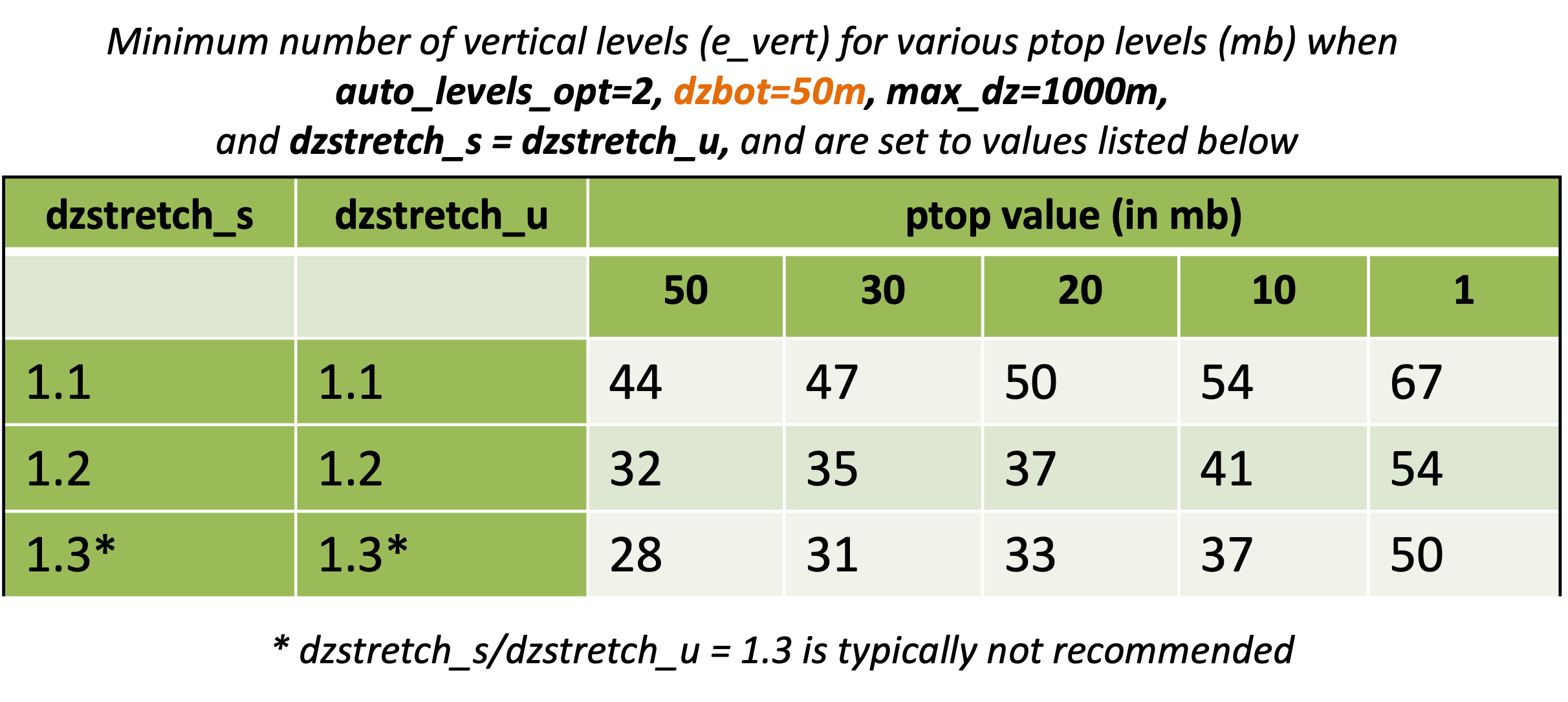
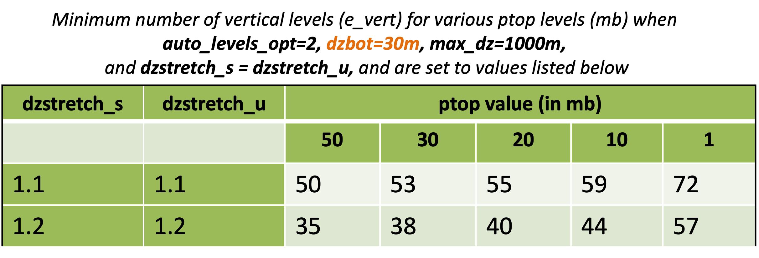
auto_levels_opt = 2 |
The default method, which uses a surface stretching factor (dzstretch_s) and an upper stretching factor (dzstretch_u) to stretch eta levels according to logP, starting from thickness dzbot, and up to the max thickness (max_dz). The stretching transitions from dzstretch_s to dzstretch_u by the time the thickness reaches max_dz/2. |
dzbot |
The thickness of the first model layer between full levels (default value is 50 m) |
max_dz |
The maximum layer thickness allowed (default is 1000 m) |
Tips for Choosing Stretching Factors
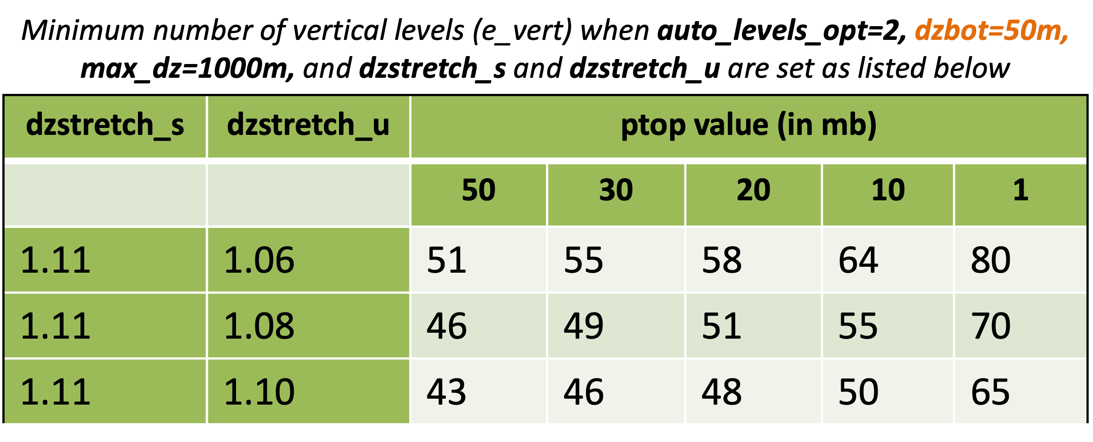
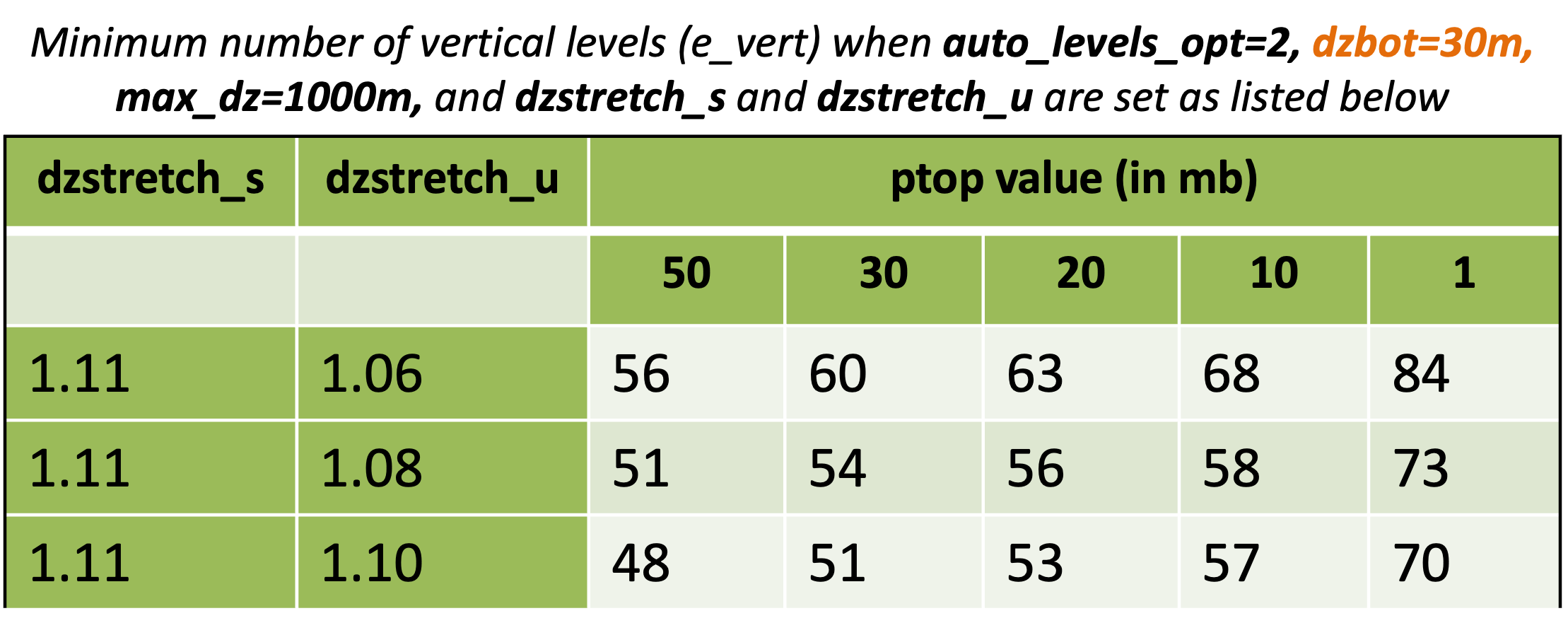
To avoid max thickness in the upper troposphere, stretching levels must extend above the tropopause before going to constant d (logP). This is accomplished by using low dzstretch_u values (but larger than ~1.02) to reach the tropopause, while also stretching fast enough to compensate the lapse rate.
Typically a thin surface layer should be used.
First choose dzbot, then max_dz (which is typically 1 km), then choose the stretching factors. Find the minimum number of levels needed to work with the other values chosen. For e.g., for more levels near the surface, use a smaller dzstretch_s.
Use trial and error, only changing one or two factors at a time, while keeping others constant.
Look at real.exe log files to see printouts of values used.
Additional resource: WRF - More Runtime Options
See the tables below for reasonable e_vert settings for dzbot=50 and dzbot=30.
Compiling Real-data Cases
See the Compiling chapter for detailed information on building both the real-data case initialization program and WRF.
Running Real-data Simulations
See Running WRF for instructions on running a real-data case.