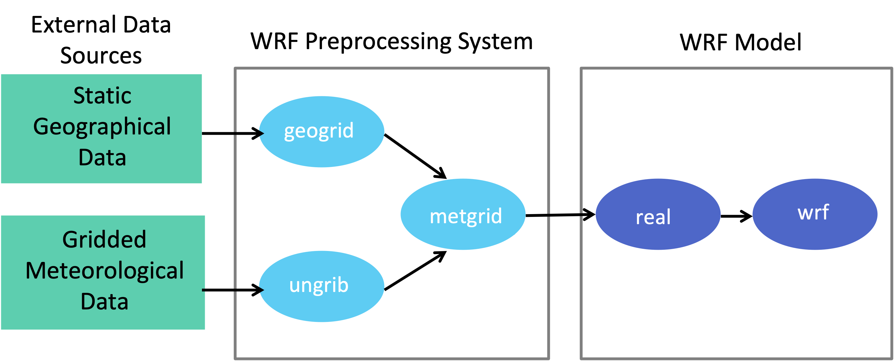
The WRF Preprocessing System (WPS)¶

The WRF Preprocessing System (WPS) is a set of three programs whose collective role is to prepare input to the real program for real-data simulations. Each program performs one stage of the preparation:

geogrid

A WPS program that defines model domains and interpolates static geographical data to the grids

ungrib

A WPS program that extracts meteorological fields from GRIB-formatted files

metgrid

A WPS program that horizontally interpolates the meteorological fields extracted by ungrib to the model grids defined by geogrid

The below figure shows data flow between the WPS programs. Each program reads parameters from a common namelist file (namelist.wps), which contains separate namelist records representing each of the programs, and a shared namelist record, which defines parameters used by more than one WPS program. Specific table files (GEOGRID.TBL, METGRID.TBL, and Vtable) are used by individual programs. They provide additional control over the programs’ operations (and generally do not need to be modified).

See the chapter on Compiling for instructions on obtaining and building the WPS code.

The Geogrid Program¶

The geogrid program is responsible for the following functions:

Defining the simulation domains - e.g., map projection, geographic location on the Earth, dimensions, and horizontal resolution
Computing latitude, longitude, and map scale factor, and Coriolis parameters at every grid point
Horizontally interpolating static (time-invariant) terrestrial fields (e.g., topography height, land use category, soil type, annual mean deep soil temperature, monthly vegetation fraction, monthly albedo, maximum snow albedo, and slope category) from global datasets, to each model grid point

Defining Model Domains¶

Model domain specifications are set by the user in the namelist.wps file, available in the top-level wps directory - specifically in the &domains namelist record.

Map Projection¶

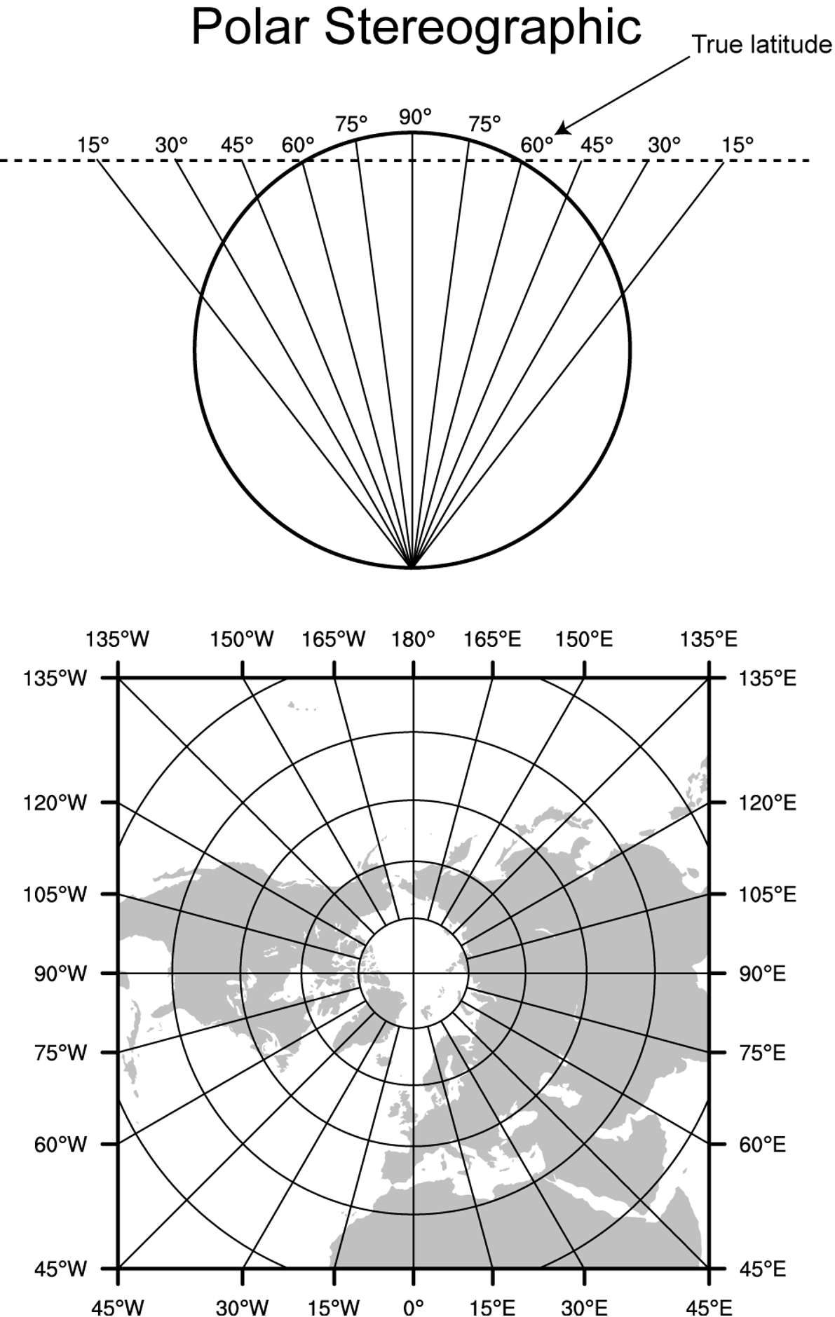
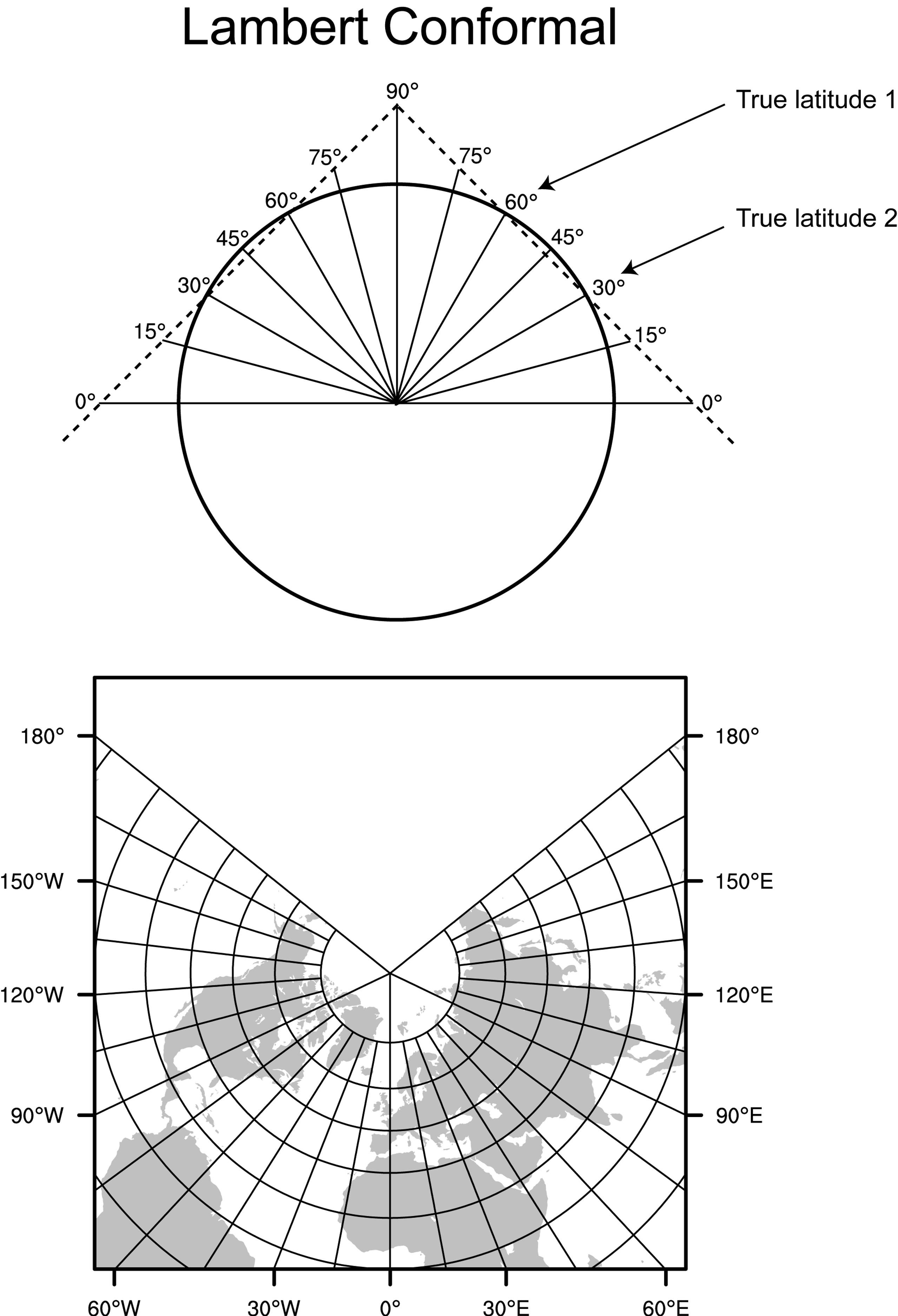
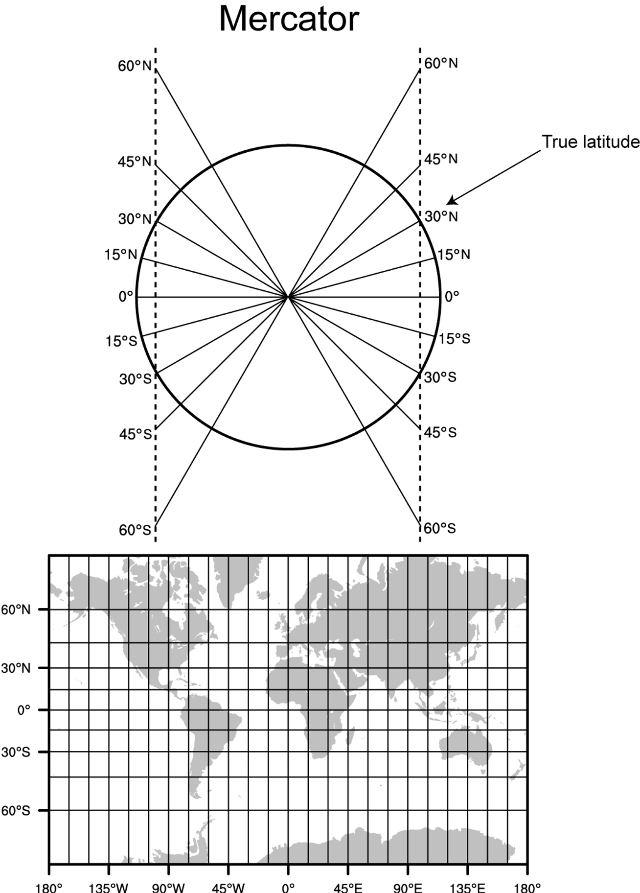
Because the earth is rougly an ellipsoid, and because WRF computational domains are defined by rectangles in the plane, a map projection must be chosen that best suites the domain. This is specified by the namelist parameter “map_proj.”The following projections, along with their namelist parameters are supported options in WPS:

Map Projection	map_proj=	Relevant Namelist Parameters	General Guidelines
Lambert Conformal	‘lambert’	truelat1 truelat2 (optional) stand_lon	well-suited for mid-latitude domains; domains cannot contain poles, nor be periodic in the west-east direction
Mercator	‘mercator’	truelat1	good for low-latitude domains or domains with predominantly west-east extent; can be used for domains periodic in the west-east direction
Polar Stereographic	‘polar’	truelat1 stand_lon	best suited for high-latitude WRF domains
Regular Latitude-Longitude, or Cylindrical Equidistant	‘lat-lon’	pole_lat pole_lon stand_lon	required for global simulations, although in its rotated aspect (i.e., when pole_lat, pole_lon, and stand_lon are changed from their default values) it can also be well-suited for regional domains anywhere on the earth’s surface

Note the “true latitude” in three of the projections in the figure below. At the true latitude, there is no distortion in the distances in the map projection, while at other latitudes, the distance on the surface of the earth is related to the distance on the surface of projection by a “map scale factor.” Ideally, the map projection and its accompanying parameters should be chosen to minimize the maximum distortion within the area covered by the model grids, since a high amount of distortion, evidenced by map scale factors significantly different from unity, can restrict the model time step more than necessary.

../../_images/wps_polar_stereographic.png

../../_images/wps_cylindrical_equidistant.png

If using the regular “lat-lon” projection for a regional domain, ensure that map scale factors in the domain’s region do not deviate significantly from unity. To do this, rotate the projection such that the area covered by the domain is located near the equator of the projection, since, for this projection, map scale factors in the x-direction are given by the cosine of the computational latitude. For example, in the figure above showing the unrotated and rotated earth, in the rotated aspect, New Zealand is located along the computational equator, and thus, the rotation used would be suitable for a domain covering New Zealand.

As a general guideline for rotating the lat-lon projection, the namelist parameters pole_lat, pole_lon, and stand_lon may be chosen according to the formulas in the following table.

Namelist Parameter Name	(ref_lat / ref_lon) in North. Hemisphere	(ref_lat
pole_lat	90.0 - ref_lat	90.0 + ref_lat
pole_lon	180.0	0.0
stand_lon	-ref_lon	180.0 - ref_lon

The Computational Grid¶

The computational grid refers to the regular latitude-longitude grid on which model computation is done, and on whose latitude circles Fourier filters are applied at high latitudes (refer to the WRF Version 4 Technical Note for details on this filtering process). The computational latitude-longitude grid is always represented with computational latitude lines running parallel to the x-axis of the model grid, and computational longitude lines running parallel to the y-axis of the grid.

If the earth’s geographic latitude-longitude grid coincides with the computational grid, a global domain shows the earth’s surface as it is normally visualized on a regular latitude-longitude grid (as is shown in the top half of the figure below). If, instead, the geographic grid does not coincide with the model computational grid, geographical meridians and parallels appear as complex curves - see the bottom half of the example below, where the geographic grid (not shown) has been rotated so that the geographic poles of the earth are no longer located at the poles of the computational grid.

When running WRF for a regional domain configuration, the location of the coarse domain is determined using the following namelist parameters:

ref_lat, ref_lon
dx, dy
e_we, e_sn

See Run the Geogrid Program for use descriptions of these variables.

Global Domains¶

Note

Although WRF supports a global domain capability, it is not usually recommended, and should be used with caution if doing so. Not all physics and diffusion options have been tested with it, and some options may not work well with polar filters. Positive-definite and monotonic advection options do not work with polar filters in a global run because polar filters can generate negative values of scalars (which implies that WRF-Chem cannot be run with positive-definite and monotonic options in a global WRF setup).

For global WRF simulations, the following applies:

The coarse domain covers the entire globe, so ref_lat and ref_lon do not apply, and dx and dy should not be specified, since the nominal grid distance is computed automatically based on the number of grid points.
The latitude-longitude, or cylindrical equidistant projection (map_proj = ‘lat-lon’) is the only WRF projection that can support a global domain.
Nested domains within a global domain must not cover any area north of computational latitude +45 or south of computational latitude -45, since polar filters are applied poleward of these latitudes (although the cutoff latitude can be changed in the WRF namelist)

Nested Domains¶

Nested Simulation

A simulation in which a coarse-resolution domain (parent) contains at least one finer-resolution domain (child) embedded. The nest receives data driven along its lateral boundaries from its parent, and depending on the settings during the WRF simulation, the nest may also provide data back to the parent.

Is a nest necessary?

Determine the size of the area necessary to fully encompass the phenomenon of interest, allowing for considerable space around all sides of that area to serve as a buffer zone.
Determine the resolution necessary to resolve the event, as well as the resolution of the input data.

A nest is necessary if:

The input data are more coarse than a factor of about five times that of the resolution required to resolve the phenomenon of interest. One or more parent(s) outside the highest-resolution domain ensures smoothness. Too much difference between the resolutions of parents to children (including the difference between parent domain and the first-guess model input resolution) can cause problems at the boundaries. For example, if needing to simulate an area at 3 km resolution, but the input data have a resolution of 1 degree (which is about 111 km), the grid ratio would be 37:1, which is much too large.
The domain size is significantly increasing computational cost. To ensure the large-scale and meso- and/or micro-scale components are all resolved, depending on the size of the phenomemon of interest, the domain may need to be fairly large. If the entire simulation area were at the highest resolution necessary, it could be computationally expensive. Consider only putting the finest resolution over the exact area of interest (with reasonable space to buffer), and using a more-coarse-resolution domain to surround it.

To specify the size and location of nests, the following namelist.wps variables must be given a value per nest. For e.g., the following is set up for a two-domain run (the coarse domain, plus a single nest):

&share
  max_dom = 2,
  start_date = '2019-09-04_12:00:00','2019-09-04_12:00:00',
  end_date   = '2019-09-04_18:00:00','2019-09-04_12:00:00',
/

&geogrid
  parent_id         =   1,   1,
  parent_grid_ratio =   1,   3,
  i_parent_start    =   1,  53,
  j_parent_start    =   1,  25,
  e_we              =  150, 220,
  e_sn              =  130, 214,
  geog_data_res     = 'default','default',
/

All namelist.wps parameters listed above need a value for each domain - i.e., the number of settings (columns) per namelist parameter should be equal to the value given for max_dom. The only other &share namelist record parameters important for nested domains are the starting and ending times, which are discussed in the The Ungrib Program section.

Note

See Run the Geogrid Program for specifics of these namelist parameters and how to use them for setting up a nested simulation.

The nesting setup in the example namelist above is illustrated in the figure below, showing how each of the above-mentioned variables is determined.

Note

To ensure that the upper-right corner of the nest’s grid is coincident with an unstaggered grid point in the parent domain, both e_we and e_sn must be one greater than some integer multiple of the nesting ratio.

For a complete description of these namelist variables, refer to WPS Namelist Variables.

Visualizing the Domain¶

plotgrids.ncl

An NCAR Graphics-based utility that can plot the locations of all nests defined in the namelist.wps file.

plotgrids.ncl, located in WPS/util operates on the namelist.wps file. It can be useful during the initial placement of domains, when namelist.wps can be edited to iteratively adjust nest locations. Run plotgrids.ncl, and determine a set of adjustments to the nest locations. To run this program from the WPS/ directory, issue:

> ncl util/plotgrids.ncl

Upon successful completion, plotgrids.ncl produces a graphics file in the chosen format (see inside the plotgrids.ncl script for output format options). The coarse domain is drawn to fill the plot frame, a map outline with political boundaries is drawn over the coarse domain, and any nested domains are drawn as rectangles outlining the extent of each nest.

Note

This utility does not work for ARW domains that use the latitude-longitude projection (i.e., when map_proj = ‘lat-lon’).

Geographic Static Fields¶

In addition to computing latitude, longitude, and map scale factors at every grid point, geogrid interpolates the following to the model grids, by default.

soil categories
land use category
terrain height
annual mean deep soil temperature
monthly vegetation fraction
monthly albedo
maximum snow albedo
slope category

Download global static datasets

If not already downloaded, click the above button to access the global static datasets. These data are time-invariant, so they only need to be downloaded once. Several data sets are available in only one resolution, but others are made available as a “full-resolution” download and as a “low-resolution” download. Generally, the low-resolution sources for static fields are suitable only for code testing and educational purposes, and any applications where model accuracy is of concern should use the full-resolution geographical data sets.

The default land use and soil category datasets provided as part of the downloaded WPS static data contain categories that are matched with the MODIS categories described in the VEGPARM.TBL, LANDUSE.TBL, and SOILPARM.TBL files available in WRF. Descriptions for these categories, in addition to all other land use and soil categories available from the WPS Geographical Static Data Downloads page, are provided in these table files, which can be found in the WRF run or test/em_real directory.

USGS and MODIS Land Use¶

By default, the geogrid program interpolates land use categories from MODIS IGBP 21-category data. However, an alternative set of land use categories based on the USGS land-cover classification may be selected.

Note

The MODIS-based 21-category land use categories are not a subset of the 24 USGS categories.

To select the 24-category USGS-based land use data, modify the geog_data_res variable in the &geogrid namelist record by prefixing each resolution of static data with the string usgs_lakes+. For example, in a two-domain configuration, where geog_data_res would ordinarily be specified as

geog_data_res = 'default', 'default',

it should instead be specifed as

geog_data_res = 'usgs_lakes+default', 'usgs_lakes+default',

This change instructs the geogrid program to look in each entry of the GEOGRID.TBL for a resolution of static data denoted by ‘usgs_lakes’, and if it is not available, to instead look for a resolution denoted by the string following the ‘+’. Thus, for the GEOGRID.TBL entry for the LANDUSEF field, the USGS-based land use data, identified with the string ‘usgs_lakes’, would be used instead of the ‘default’ resolutions (or source) of land use data in the example above; for all other fields, the ‘default’ resolutions would be used. When none of the resolutions specified for a domain in geog_data_res are found in a GEOGRID.TBL entry, the resolution denoted by ‘default’ will be used.

Important

To change from the default 21-class MODIS land-use data, set num_land_cat=21 in the &physics WRF namelist.input record. For 24-class USGS data, set num_land_cat=24.

GEOGRID.TBL¶

GEOGRID.TBL

A text file (located in wps/geogrid) that defines parameters of each data set to be interpolated by geogrid.

Each data set is defined in a separate section, with sections being delimited by a line of equality symbols (e.g., ==============). Within each section, there are specifications, each of which has the form of keyword=value. Some keywords are required in each data set section, while others are optional; some keywords are mutually exclusive with other keywords. Below, the possible keywords and their expected range of values are described.

Variable Name	Default Value	Description
name	no default	A character string specifying the name that will be assigned to the interpolated field upon output
priority	no default	An integer specifying the priority that the data source identified in the table section takes with respect to other sources of data for the same field. If a field has n sources of data, there must be n separate table entries for the field, each of which must be given a unique priority value in the range [1, n]
dest_type	no default	A character string, either categorical or continuous, indicating whether the interpolated field from the data source given in the table section is to be treated as a continuous or a categorical field
interp_option	no default	A sequence of one or more character strings, which are the names of interpolation methods to be used when horizontally interpolating the field. Available interpolation methods are: average_4pt average_16pt wt_average_4pt wt_average_16pt nearest_neighbor four_pt sixteen_pt search(r) average_gcell(r) For the search method, the optional argument r specifies the maximum search radius in units of grid points in the grid of the source data (the default is 1200 points). For the grid cell average method (average_gcell), optional argument r specifies the minimum ratio of source data resolution to simulation grid resolution at which the method will be applied; unless specified, r = 0.0, and the option is used for any ratio. When a sequence of two or more methods are given, methods should be separated by a + sign
smooth_option	<null> (i.e., no smoothing applied)	A character string giving the smoothing method to be applied to the field after interpolation. Available smoothing options are: 1-2-1 smth-desmth smth-desmth_special (ARW only)
smooth_passes	1	If smoothing is to be performed on the interpolated field, smooth_passes specifies an integer number of passes of the smoothing method to apply to the field
rel_path	no default	A character string specifying the path relative to the path given in the namelist variable geog_data_path. A specification is of the general form RES_STRING:REL_PATH, where RES_STRING is a character string identifying the source or resolution of the data in some unique way and may be specified in the namelist variable geog_data_res, and REL_PATH is a path relative to geog_data_path where the index and data tiles for the data source are found. More than one rel_path specification may be given in a table section if there are multiple sources or resolutions for the data source, just as multiple resolutions may be specified (in a sequence delimited by + symbols) for geog_data_res. See also abs_path
abs_path	no default	A character string specifying the absolute path to the index and data tiles for the data source. A specification is of the general form RES_STRING:ABS_PATH, where RES_STRINGe is a character string identifying the source or resolution of the data in some unique way and may be specified in the namelist variable geog_data_res, and ABS_PATH is the absolute path to the data source’s files. More than one abs_path specification may be given in a table section if there are multiple sources or resolutions for the data source, just as multiple resolutions may be specified (in a sequence delimited by + symbols) for geog_data_res. See also rel_path
output_stagger	M	A character string specifying the grid staggering to which the field is to be interpolated. Possible values are U, V, and M
landmask_water	<null> (i.e., a landmask will not be computed from the field)	One or more comma-separated integer values giving the indices of the categories within the field that represent water. When landmask_water is specified in the table section of a field for which dest_type=categorical, the LANDMASK field will be computed from the field using the specified categories as the water categories. The keywords landmask_water and landmask_land are mutually exclusive
landmask_land	<null> (i.e., a landmask will not be computed from the field)	One or more comma-separated integer values giving the indices of the categories within the field that represent land. When landmask_water is specified in the table section of a field for which dest_type=categorical, the LANDMASK field will be computed from the field using the specified categories as the land categories. The keywords landmask_water and landmask_land are mutually exclusive
masked	<null> (i.e., a landmask will not be computed from the field)	A character string (either land or water) indicating that the field is not valid at land or water points, respectively. If the masked keyword is used for a field, those grid points that are of the masked type (land or water) will be assigned the value specified by fill_missing
fill_missing	1.00E+20	A real value used to fill in any missing or masked grid points in the interpolated field
halt_on_missing	no	A character string (either yes or no) indicating whether geogrid should halt with a fatal message when a missing value is encountered in the interpolated field
dominant_category	<null> (i.e., no dominant category will be computed from the fractional categorical field)	When specified as a character string, geogrid computes the dominant category from the fractional categorical field, and outputs the dominant category field with the name specified by the value of dominant_category. This option can only be used for fields with dest_type=categorical
dominant_only	<null> (i.e., no dominant category will be computed from the fractional categorical field)	When specified as a character string, geogrid computes the dominant category from the fractional categorical field and outputs the dominant category field with the name specified by the value of dominant_only. When dominant_only is used, the fractional categorical field will not appear in the geogrid output. This option can only be used for fields with dest_type=categorical
df_dx	<null> (i.e., no derivative field is computed)	When df_dx is assigned a character string value, geogrid computes the directional derivative of the field in the x-direction using a central difference along the interior of the domain, or a one-sided difference at the boundary of the domain; the derivative field will be named according to the character string assigned to the keyword df_dx
df_dy	<null> (i.e., no derivative field is computed)	When df_dy is assigned a character string value, geogrid computeis the directional derivative of the field in the y-direction using a central difference along the interior of the domain, or a one-sided difference at the boundary of the domain; the derivative field will be named according to the character string assigned to the keyword df_dy
z_dim_name	no default	For 3-dimensional output fields, a character string giving the name of the vertical dimension, or z-dimension. A continuous field may have multiple levels, and thus be a 3-dimensional field, and a categorical field may take the form of a 3-dimensional field if it is written out as fractional fields for each category
flag_in_output	<null> (i.e., no flag will be written for the field)	A character string giving the name of a global attribute which will be assigned a value of 1 and written to the geogrid output
optional	no	A character string (either yes or no) indicating whether the dataset identified by the resolution specified in the geog_data_res namelist option is optional. If an entry in GEOGRID.TBL is optional and if the specified resolution of data cannot be read, geogrid will print a message indicating that the dataset was not interpolated and continue; otherwise, if the entry is not optional and the specified resolution of data cannot be read, geogrid will halt with an error. It is possible for different priority level entries for the same field to specify different values of the optional keyword, e.g., the priority=2 entry for a field can be optional, while the priority=1 entry can be non-optional (i.e., optional=no)

When geogrid is run, it looks for a table with the name “GEOGRID.TBL.” By default, this table is linked to GEOGRID.TBL.ARW, as is shown below. To use a different table, link that table to the expected name GEOGRID.TBL.

> ls -ls geogrid/GEOGRID.TBL

  lrwxrwxrwx  1         15  GEOGRID.TBL -> GEOGRID.TBL.ARW

Index Options¶

Related to the GEOGRID.TBL are the index files associated with each static data set.

index

A file for each static data set that defines parameters specific to that data set

Specifications in an index file are of the form keyword=value. Below are possible keywords and their possible values.

Variable Name	Default Value	Description
projection	no default	A character string specifying the data’s projection; options are lambert polar mercator regular_ll albers_nad83 polar_wgs84
type	no default	A character string (either categorical or continuous) that determines whether the data should be interpreted as a continuous field or as discrete indices. For categorical data represented by a fractional field for each possible category, type should be set to continuous
signed	no	A character string (either yes or no) indicating whether the values in the data files (which are represented as integers) are signed in “two’s complement” form
units	no default	A character string enclosed in quotation marks (“) specifying the units of the interpolated field; the string will be written to the geogrid output files as a variable time-independent attribute
description	no default	A character string enclosed in quotation marks (“) giving a short description of the interpolated field; the string will be written to the geogrid output files as a variable time-independent attribute
dx dy	no default	A real value giving the data set’s grid spacing in the x- or y-direction (respectively). If projection is one of lambert, polar, mercator, albers_nad83, or polar_wgs84, grid spacing is given in meters; if the projection is regular_ll, grid spacing is given in degrees
known_x known_y	1	A real value specifying the i- or j-coordinate (respectively) of an (i,j) location corresponding to a (latitude, longitude) location that is known in the projection
known_lat known_lon	no default	A real value specifying the latitude or longitude (respectively) of a (latitude, longitude) location that is known in the projection
stdlon	no default	A real value specifying the longitude that is parallel with the y-axis in conic and azimuthal projections
truelat1	no default	A real value specifying the first true latitude for conic projections or the only true latitude for azimuthal projections
truelat2	no default	A real value specifying the second true latitude for conic projections
wordsize	no default	An integer giving the number of bytes used to represent the value of each grid point in the data files
tile_x tile_y	no default	An integer specifying the number of grid points in the x- or y-direction (respectively), excluding any halo points, for a single tile of source data
tile_z	no default	An integer specifying the number of grid points in the z-direction for a single tile of source data; tile_z is an alternative to using the pair of keywords tile_z_start and tile_z_end, and when tile_z is used, the starting z-index is assumed to be 1
tile_z_start tile_z_end	no default	An integer specifying the starting or ending index (respectively) in the z-direction of the array in the data files. These two keywords must be used together.
category_min category_max	no default	For categorical data (type=categorical), an integer specifying the minimum or maximum (respectively) category index that is found in the data set. These two keywords must be used together.
tile_bdr	0	An integer specifying the halo width, in grid points, for each tile of data
missing_value	no default	A real value that, when encountered in the data set, should be interpreted as missing data
scale_factor	1	A real value by which data should be scaled (through multiplication) after being read in as integers from tiles of the data set
row_order	bottom_top	A character string (either bottom_top or top_bottom) specifying whether the rows of the data set arrays were written proceeding from the lowest-index row to the highest (bottom_top) or from highest to lowest (top_bottom). This keyword may be useful when utilizing some USGS data sets, which are provided in top_bottom order
endian	big	A character string (either big or little) specifying whether the values in the static data set arrays are in big-endian or little-endian byte order
iswater	16	An integer specifying the land use category of water
islake	-1 (i.e., no separate inland water category)	An integer specifying the land use category of inland water bodies
isice	24	An integer specifying the land use category of ice
isurban	1	An integer specifying the land use category of urban areas
isoilwater	14	An integer specifying the soil category of water
mminlu	MODIFIED_IGBP_MODIS_NOAH	A character string enclosed in quotation marks (“) indicating which section of WRF’s LANDUSE.TBL and VEGPARM.TBL will be used when looking up parameters for land use categories during wrf.exe
filename_digits	5	An integer specifying the number of digits used in the names of data tiles. Possible values are 5 or 6.

Writing Static Data to the Geogrid Binary Format¶

The static geographical data sets that are interpolated by the geogrid program are stored as regular 2-d and 3-d arrays written in a simple binary raster format. Users with a new source for a given static field can ingest their data with WPS by writing the data set into this binary format. The geogrid format supports

single-level and multi-level continuous fields
categorical fields represented as dominant categories
categorical fields given as fractional fields for each category

The simplest of these field types, in terms of representation in the binary format, is a categorical field given as a dominant category at each source grid point, an example of which is the 30-second USGS land use data set.

../../_images/wps_geogrid_binary_format.png

Categorical field given as dominant categories

Data must first be stored in a regular 2-d array of integers, with each integer giving the dominant category at the corresponding source grid point.
Given this array, the data are written to a file, row-by-row, beginning at the bottom, or southern-most, row.
For example, in the figure above, the elements of the n ‘ m array are written in the order x11, x12, …, x1m, x21, …, x2m, …, xn1, …, xnm.
When written to the file, every element is stored as a 1-, 2-, 3-, or 4-byte integer in big-endian byte order (i.e., for the 4-byte integer ABCD, byte A is stored at the lowest address and byte D at the highest),
Every element in a file must use the same number of bytes for its storage, and it is advantageous to use the fewest number of bytes needed to represent the complete range of values in the array.
When writing the binary data to a file, no header, record marker, or additional bytes should be written.
For example, a 2-byte 1000 ´ 100 array should result in a file whose size is exactly 2,000,000 bytes. Since Fortran unformatted writes add record markers, it is not possible to write a geogrid binary-formatted file directly from Fortran; instead, the C routines in read_geogrid.c and write_geogrid.c (in the geogrid/src directory) should be called when writing data, either from C or Fortran code.

Note

Little-endian files may be used by setting endian=little in the index file for the data set

Fields of continuous, or real, values
Like dominant-category fields, single-level continuous fields are first organized as a regular 2-d array, then written, row-by-row, to a binary file. However, because a continuous field may contain non-integral or negative values, the storage representation of each element within the file is slightly more complex.

All elements in the array must first be converted to integral values. This is done by first scaling all elements by a constant, chosen to maintain the required precision, and then removing any remaining fractional part through rounding.
For example, if three decimal places of precision are required, the value -2.71828 would need to be divided by 0.001 and rounded to -2718.
Following the conversion of all array elements to integral values, if any negative values are found in the array, a second conversion must be applied: if elements are stored using 1 byte each, then 2⁸ is added to each negative element; for storage using 2 bytes, 2¹⁶ is added to each negative element; for storage using 3 bytes, 2²⁴ is added to each negative element; and for storage using 4 bytes, a value of 2³² is added to each negative element. Note that no conversion is applied to positive elements. Finally, the resulting positive, integral array is written as in the case of a dominant-category field.

Multi-level continuous fields

For an n ´ m ´ array, conversion to a positive, integral field is first performed as described above.
Then, each n ´m sub-array is written contiguously to the binary file as before, beginning with the smallest r-index.

Categorical fields, given as fractional fields for each possible category, can be thought of as multi-level continuous fields, where each level k, 1 <= k <= r, is the fractional field for category k.

Geogrid binary file naming convention
When writing a field to a file in the geogrid binary format, the user should adhere to the naming convention used by the geogrid program, which expects data files to have names of the form xstart-xend.ystart-yend, where xstart, xend, ystart, and yend are five-digit positive integers specifying, respectively, the starting x-index of the array contained in the file, the ending x-index of the array, the starting *y-index of the array, and the ending y-index of the array; here, indexing begins at 1, rather than 0. So, for example, an 800 ´ 120 array (i.e., 800 rows and 1200 columns) might be named 00001-01200.00001-00800.

When a data set is given in several pieces, each piece may be formed as a regular rectangular array, and each array may be written to a separate file. In this case, the relative locations of the arrays are determined by the range of x- and y-indices in the file names for each of the arrays.

Important

Every tile in a data set must have the same x- and y-dimensions*
Tiles of data within a data set must not overlap
All tiles must start and end on multiples of the index ranges. For example, the global 30-second USGS topography data set is divided into arrays of dimension 1200 ´ 120, with each array containing a 10-degree ´ 10-degre piece of the data set; the file whose south-west corner is located at (90S, 180W) is named 00001-01200.00001-01200, and the file whose north-east corner is located at (90N, 180E) is named 42001-43200.20401-21600.

If splitting a data set into multiple tiles, when the number of grid points in, say, the x-direction is not evenly divided by the number of tiles in the x-direction, then the last column of tiles must be padded with a flag value (specified in the index file using the missing_value keyword - see Index Options above) so that all tiles have the same dimensions. For example, if a data set has 2456 points in the x-direction, and three tiles in the x-direction will be used, the range of x-coordinates of the tiles might be 1-820, 821-1640, and 1641-2460, with columns 2457 through 2460 being filled with a flag value.

Since the starting and ending indices must have five digits, a field cannot have more than 99999 data points in either of the x- or y-directions. In case a field has more than 99999 data points in either dimension, the data set can be split into several smaller data sets, which will be identified separately to geogrid. For example, a very large global data set may be split into data sets for the Eastern and Western hemispheres.

Creating an Index File for the Static Dataset
Besides the binary data files, geogrid requires one extra metadata file per data set. This metadata file is always named index, and thus, two data sets cannot reside in the same directory. This metadata file is the first file geogrid looks for when processing a data set, and the contents of the file provide all of the information necessary for constructing names of possible data files. The contents of an example index file are given below.

type = continuous
     signed = yes
     projection = regular_ll
     dx = 0.00833333
     dy = 0.00833333
     known_x = 1.0
     known_y = 1.0
     known_lat = -89.99583
     known_lon = -179.99583
     wordsize = 2
     tile_x = 1200
     tile_y = 1200
     tile_z = 1
     tile_bdr=3
     units="meters MSL"
     description="Topography height"

See the Index Options section for a complete listing of keywords that may appear in an index file, along with the meaning of each keyword.

Gravity Wave Drag Scheme Static Data¶

The WRF gravity wave drag by orography (GWDO) scheme requires ten static fields that are interpolated by the geogrid program (regardless of whether the GWDO scheme will be used in the model). When the GWDO scheme is not used, the fields are ignored in WRF. Otherwise, these fields should be interpolated from a source data resolution slightly coarser in resolution than the model grid. Five resolutions of GWDO static data are available: 2-degree, 1-degree, 30-minute, 20-minute, and 10-minute, denoted by the strings ‘2deg’, ‘1deg’, ‘30m’, ‘20m’, and ‘10m’, respectively.

The setting for geog_data_res in the namelist.wps &geogrid record determines which resolution to interpolate from. For example, in a 48-km grid spacing model configuration, geog_data_res is typically specified as

geog_data_res = 'default',

However, if the GWDO scheme is employed, the finest resolution of GWDO static data that is still lower in resolution than the model grid is the 30-minute data, in which case the setting should be

geog_data_res = '30m+default',

If none of ‘2deg’, ‘1deg’, ‘30m’, or ‘20m’ are specified in combination with other static data resolutions, the default resolution of ‘10m’ GWDO static data is used. Note that if 10-minute resolution GWDO data are used, but a different resolution is desired for other static fields (e.g., topography height), ‘10m’ should be emitted from the value given to geog_data_res, since specifying

geog_data_res = '10m+30s',

for example, would cause geogrid to use the 10-minute data in preference to the 30-second data for the non-GWDO fields, such as topography height and land use category, as well as for the GWDO fields.

NLCD Urban Fraction Field¶

Note

An urban fraction field that is prepared based on 30-meter NLCD 2011 land cover for the continental United States is available from WPS Geographical Static Data Downloads under the section for “optional fields”. The details below may be helpful for preparing urban fraction fields for other regions.

To create a more inhomogeneous and detailed urban fraction field for use with NUDAPT, high-resolution land cover information is obtainable from the National Land Cover Database (NLCD) through the Multi-Resolution Land Characteristics Consortium. To generate the urban fraction field (FRC_URB2D) in WRF:

1. Download the NLCD data over the region covered by the WRF domain
Download NLCD data. Either of the 1992, 2001, or 2006 data sets may be used. After selecting an area to download, select GeoTIFF format in the “Request Summary Page” by clicking on Modify Data Request. If available, data may instead be downloaded in BIL format, in which case the format conversion described in the next step can be skipped.

2. Convert the data into the binary format used by geogrid

Unpack the archive, which should yield a directory that includes a .tif file and a .tfw file, among others. For the information in the GeoTIFF file to be useful, the .tif image must be converted into the binary format used by the WPS (see Writing Static Data to the Geogrid Binary Format for reference), which can be accomplished using the GDAL translation tool, gdal_translate, by issuing the command

> gdal_translate -of ENVI foo.tif data.bil

Here,

foo.tif
the name of the GeoTIFF image that was downloaded in Step 1.
ENVI
the simple binary raster output format that matches the format used by geogrid.
data.bil
the resulting file after converting GeoTIFF to a binary file

data.bil must be renamed to 00001-ncols.00001-nrows, where ncols is the number of columns (in i5.5 format) and nrows is the number of rows (also in i5.5 format) in the image; these values should be printed to the screen when gdal_translate is run.

3. Extract only the urban categories to a new urban fraction field
Use this converter program to extract the urban categories from the binary tile and write a new tile of data containing urban fraction. The output file of this converter should be copied over the original land use tile, i.e., the urban fraction file should be renamed to 00001-ncols.00001-nrows, where ncols is the number of columns (in i5.5 format) and nrows is the number of rows (also in i5.5 format) in the tile, as in Step 2.

4. Create an index metadata file for the urban fraction data
(see Index Options)

A .tfw file should exist in the directory created by unpacking the land use data. The last two lines in this file give the location of the north-west corner of the data tile, which is used in the index file for variables known_lat and known_lon. If this location is given as (x,y) coordinates, in meters, then this coordinate converter utility may be used to convert to (latitude, longitude), which is required by the index file. The basic index file should contain the following elements:

type=continuous
projection=albers_nad83
dx=30.0
dy=30.0
known_x=1.0
known_y=2351.0            # <- edit
known_lat =   40.096571   # <- edit
known_lon = -105.405615   # <- edit
truelat1=29.5
truelat2=45.5
stdlon=-96.0
wordsize=1
scale_factor=0.01
row_order=top_bottom
tile_x=2407               # <- edit
tile_y=2351               # <- edit
tile_z=1
units="unitless"
description="urban fraction"

5. Add the following entry to the GEOGRID.TBL file
GEOGRID.TBL is found in WPS/geogrid. This should be added before re-running the geogrid.exe program:

===============================
name=FRC_URB2D
priority=1
dest_type=continuous
fill_missing = 0.
interp_option=default: average_gcell(1.0)+four_pt
abs_path=default:/path/to/dataset/
===============================

The path to the created data set (step 3) and index files (step 4) should be substituted for “path/to/dataset/” in the entry above.

Alternative Initialization of Lake SSTs¶

By default, metgrid interpolates the sea surface temperature (SST) field - both for oceans and lakes - from the intermediate files to all water points in the WRF domain. However, if the lakes that are resolved in the WRF domain are not resolved in the GRIB data, and especially if those lakes are geographically distant from resolved water bodies, SST over lakes will most likely be extrapolated from the nearest resolved water bodies in the GRIB data, which can lead to lake SST values that are either unrealistically warm or cold.

Without a higher-resolution SST field for metgrid to use, one alternative to extrapolating lake SST values is to manufacture a “best guess” at the lake SSTs, using a combination of a special land use data set that distinguishes between lakes and oceans, and a field to be used as a proxy for SST over lakes. This relays to WRF’s real pre-processing where to use the manufactured SST field, instead of the interpolated SST field from the GRIB data.

The alternative procedure for initializing lake SSTs is summarized in the following steps:

Before running geogrid, ensure that geog_data_res in the &geogrid namelist record indicates either the MODIS-based or USGS-based land use data that includes inland water bodies. For example, for a two-domain configuration, the following setting instructs geogrid to use the USGS-based land use data for both domains
```
geog_data_res = 'usgs_lakes+default', 'usgs_lakes+default',
```
Afterward, geogrid output should include a separate category for inland water bodies, instead of the general water category used for oceans and seas. The lake category is identified by the global attribute ISLAKE, which should be set to either 28 (USGS-based data) or 21 (MODIS-based data). See, e.g., the list of WPS Output, where a value of -1 for ISLAKE indicates there is no separate lake category.
After running ungrib, use the avg_tsfc.exe utility to create an intermediate file containing daily-average surface air temperature, which substitutes SST only over lakes in the real program
Before running metgrid, point to the TAVGSFC file created in the previous step by setting constants_name=’TAVGSFC’ in the &metgrid namelist record.
Run WRF’s real.exe program after setting the number of land categories (num_land_cat) in the &physics namelist.input record to the value of the global attribute NUM_LAND_CAT in the metgrid output. If ISLAKE in the metgrid output indicates the use of a special lakes land use category, the real program substitutes TAVGSFC for SST only over those grid points whose category matches the lake category; additionally, real.exe changes the land use category of lakes back to the general water category (the category used for oceans), since neither the LANDUSE.TBL nor the VEGPARM.TBL files contain an entry for a lake category.

The Ungrib Program¶

The ungrib program performs the following functions:

Reading GRIB-formatted data files
“Degribbing” the data
Writing the data in a simple format called the intermediate format (see Writing Meteorological Data to the Intermediate Format for details).

GRIB Files

Files containing time-varying meteorological fields, typically from another regional or global model (e.g., NCEP’s GFS model).

The ungrib program can read GRIB Edition 1 and, if compiled with a “GRIB2” option, GRIB Edition 2 files.

Ungrib can write intermediate data files in any one of three user-selectable formats:

WPS : a format containing additional information useful for the downstream programs
SI : an outdated intermediate format of the WRF system
MM5 : a format that allows ungrib to provide GRIB2 input to the MM5 modeling system.

Note

Any of these formats may be used by WPS to initialize WRF, although the WPS format is recommended.

Vtable¶

GRIB files typically contain more fields than are needed to initialize WRF. GRIB formatting uses codes to identify the variables and levels in the files. Ungrib uses tables - called Vtables, for “variable tables” - to define which fields to extract from the GRIB file and write to the intermediate format. Details about the codes can be found in the WMO GRIB documentation and in documentation from the originating center. The following Vtables (found in ungrib/Variable_Tables) for common GRIB model output files are provided with the ungrib software:

Vtable Name	For Use With	Input Format
Vtable.AFWAICE	Air Force Weather Agency (AFWA) ice fields	Grib1
Vtable.AGRMETSNOW	AFWA snow fields	Grib1
Vtable.AGRMETSOIL	AFWA soil fields with soil category	Grib1
Vtable.AGRMETSOIL2	AFWA soil fields with land use & vegetation categories, and green vegetation fraction	Grib1
Vtable.AGRWRF	AFWA	Grib1
Vtable.ARW.UPP	WRF output that has been processed by UPP; on eta/sigma levels	Grib1/Grib2
Vtable.ARWp.UPP	WRF output that has been processed by UPP; on pressure levels	Grib1/Grib2
Vtable.AVN0P5WRF	AFWA	Grib1
Vtable.AWIP	NAM AWIP	Grib1
Vtable.CFSR	NCEP Climate Forecast System Reanalysis	Grib1/Grib2
Vtable.CFSR_mean	NCEP Climate Forecast System Reanalysis monthly mean	Grib1/Grib2
Vtable.ECMWF	European Centre for Medium-range Weather Forecasts (ECMWF)	Grib1
Vtable.ECMWF_sigma	ECMWF hybrid-level	Grib1
Vtable.ERA-interim.ml	ERA-interim model-level	Grib1
Vtable.ERA-interim.pl	ERA-interim pressure-level	Grib1
Vtable.GFDL	GFDL	Grib1
Vtable.GFS	GFS and GFS-FNL Pressure-level data	Grib1/Grib2
Vtable.GFSENS	GFS Ensemble	Grib1/Grib2
Vtable.GODAS	NCEP’s Global Ocean data assimilation system	Grib1
Vtable.GSM	GSM data	Grib1
Vtable.JMAGSM	Japanese Meteorological Agency Global Spectral Model	Grib1/Grib2
Vtable.NAM	North American Model	Grib1/Grib2
Vtable.NARR	North American Regional Reanalysis	Grib1
Vtable.NCEP2	NCEP/DOE Reanalysis (Reanalysis-2)	Grib1
Vtable.NNRP	NCEP/NSF NCAR Reanalysis	Grib1
Vtable.NOGAPS	Navy Operational Global Atmospheric Prediction System	Grib1/Grib2
Vtable.NOGAPS_needs_GFS_soil	Navy Operational Global Atmospheric Prediction System Surface/Soil Data	Grib1/Grib2
Vtable.NavySST	AFWA sea-surface temperature data	Grib1
Vtable.RAP.hybrid.ncep	Rapid refresh hybrid-vertical coordinate data	Grib1/Grib2
Vtable.RAP.pressure.ncep	Rapid refresh pressure-level data	Grib1/Grib2
Vtable.RAP.sigma.gsd	NOAA ESRL Global Systems Division sigma-level data	Grib1/Grib2
Vtable.RUCb	Rapid Update Cycle hybrid coordinate data	Grib1/Grib2
Vtable.RUCp	Rapid Update Cycle pressure-level data	Grib1/Grib2
Vtable.SREF	NCEP’s SREF data	Grib1/Grib2
Vtable.SST	General sea-surface temperature data	Grib1/Grib2
Vtable.TCRP	Twentieth Century Global Reanalysis, Version 2	Grib1
Vtable.UKMO_ENDGame	UK Met Office Endgame data	Grib1/Grib2
Vtable.UKMO_LANDSEA	UK Met Office landsea data	Grib1/Grib2
Vtable.UKMO_no_heights	UK Met Office data, with no heights	Grib1/Grib2
Vtable.raphrrr	RAP High-resolution Rapid Refresh	Grib1/Grib2

Creating and Editing Vtables¶

Although Vtables are provided for many common data sets, every possible source of meteorological data in GRIB format is not accounted for, and users may be required to create a new Vtable. The recommended method for doing so is using an existing Vtable as an example.

Each Vtable contains either seven or eleven fields, depending on whether the Vtable is for a GRIB Edition 1 or a GRIB Edition 2 data source, respectively. Vtable fields fall into one of three categories:

fields that describe how the data are identified within the GRIB file
fields that describe how the data are identified by the ungrib and metgrid programs
fields specific to GRIB Edition 2

Each variable occupies one or more lines in the Vtable, with multiple lines for data that are split among different level types - for example, surface level and upper-air levels. The fields required for a line, or entry, in the Vtable depends on the specifics of the field and level.

The first group of fields - those that describe how the data are identified within the GRIB file - are given under the column headings of the Vtable shown below, followed by their descriptions.

GRIB1| Level| From |  To  |
Param| Type |Level1|Level2|
-----+------+------+------+

GRIB1 Param
Specifies the GRIB code for the meteorological field, which is a number unique to that field within the data set. Different data sets may use different GRIB codes for the same field. To determine a field’s GRIB code, use the g1print.exe or g2print.exe utility program (found in WPS/util).
Level Type, From Level1, From Level2
Given a GRIB code, these fields are used to specify on which levels a field may be found. The g1print.exe or g2print.exe program (found in WPS/util)may be used to find values for the level fields. The level field meanings are dependent on the Level Type field and are summarized in the following table.

Level	Level Type	From Level1	To Level2
Upper-air	100		(blank)
Surface	1	0	(blank)
Sea-level	102	0	(blank)
Levels at a specified height AGL	105	Height, in meters, of the level above ground	(blank)
Fields given as layers	112	Starting level for the layer	Ending level for the layer

When layer fields (Level Type 112) are specified, the starting and ending points for the layer use units dependent on the field itself; appropriate values may be found with the g1print.exe and g2print.exe utility programs (found in WPS/util).

The second group of fields in a Vtable - those that describe how the data are identified within the metgrid and real programs, falls under the column headings shown below, followed by their descriptions.

| metgrid  | metgrid | metgrid                                 |
| Name     |  Units  | Description                             |
+----------+---------+-----------------------------------------+

metgrid Name
Determines the variable name that will be assigned to a meteorological field when it is written to the intermediate files by ungrib. This name must match an entry in the METGRID.TBL so the metgrid program can determine how the field is to be horizontally interpolated.
metgrid Units
Specify the units for a field
metgrid Description
Specifies a short description for the field. If no description is given, that field will not be written out to the intermediate files.

The final group of fields, which provide GRIB2-specific information, are found under the column headings below.

|GRIB2|GRIB2|GRIB2|GRIB2|
|Discp|Catgy|Param|Level|
+-----------------------+

GRIB2 fields are only needed in a Vtable used for GRIB Edition 2 data sets, although having these fields in a Vtable does not prevent the Vtable from being used for GRIB Edition 1 data. For example, Vtable.GFS contains GRIB2 Vtable fields, but is used for both 1-degree (GRIB1) GFS and 0.5-degree (GRIB2) GFS data sets. Since Vtables are provided for most known GRIB Edition 2 data sets, the corresponding Vtable fields are not described here.

Required Input for Running WRF¶

To successfully initialize a WRF simulation, the real.exe pre-processor requires a minimum set of meteorological and land-surface fields in the output from the metgrid.exe program. These required fields must be available in the intermediate files processed by metgrid.exe. The set of required fields is described in the table below.

Field Name in Intermediate File	Units	Description	Notes
TT	K	3-d air temperature
RH	%	3-d relative humidity	Not needed if 3-d SPECHUMD is available
SPECHUMD	kg kg^-1	3-d specific humidity	Not needed if 3-d RH is available
UU	m s^-1	3-d wind u-component
VV	m s^-1	3-d wind v-component
GHT	m	3-d geopotential height
PRESSURE	Pa	3-d pressure	Only neede for non-isobaric data sets
PSFC	Pa	Surface pressure
PMSL	Pa	Mean sea-level pressure
SKINTEMP	K	Skin temperature
SOILHGT	m	Soil height
TT	K	2-meter air temperature
RH	%	2-meter relative humidity	Not needed if 2-meter SPECHUMD is available
SPECHUMD	kg kg^-1	2-meter specific humidity	Not needed if 2-meter RH is available
UU	m s^-1	10-meter wind u-component
VV	m s^-1	10-meter wind v-component
LANDSEA	fraction	Land-sea mask	0=water; 1=land
SMtttbbb	m³ m^-3	Soil moisture	‘ttt’ is the layer top depth in cm, and ‘bbb’ is the layer bottom depth in cm
STtttbbb	K	Soil temperature	‘ttt’ is the layer top depth in cm, and ‘bbb’ is the layer bottom depth in cm
SOILMmmm	kg m^-3	Soil moisture	‘mmm’ is the level depth in cm, not needed if SMtttbbb is available
SOILTmmm	K	Soil temperature	‘mmm’ is the level depth in cm, not needed if SMtttbbb is available

Using Multiple Meteorological Data Sources¶

The Metgrid Program is capable of interpolating data from multiple sources of time-varying, meteorological data, which may be useful when two or more complementary data sets must be combined to produce the full input data needed by real.exe. To do this, the ungrib program must be run once per data source.

Multiple Data Types from a Single Data Source¶

For example, a user is utilizing the North American Regional Reanalysis (NARR) data set, which is split into the following separate GRIB files: 3-dimensional atmospheric data, surface data, and fixed-field data. The following instructions describe the method for processing the three different GRIB files.

Note

Refer to Running the WPS for detailed steps to run.

Process the 3D atmospheric data

Use the link_grib.csh script to link the 3D atmospheric data files to the WPS directory.
Link the NARR Vtable to the filename Vtable
Edit the prefix namelist.wps parameter in the &ungrib record to specify these data. This setting is the user’s choice, and can be a prefix for the ungrib.exe output intermediate files, or can include a path to the files created by ungrib.
```
&ungrib
  out_format = 'WPS',
  prefix = 'NARR_3D',
/
```
Run ungrib.exe, which should produce the following files (with a suitable substitution for the appropriate dates):
```
NARR_3D:2024-08-16_12
NARR_3D:2024-08-16_15
NARR_3D:2024-08-16_18
...
```

Process the surface field data

Use the link_grib.csh script to link the surface data files to the WPS directory.
Because the NARR Vtable includes surface field information, there is no need to link to a different Vtable.
Change the prefix namelist parameter (in &ungrib) to something that will distinguish the surface intermediate files from the 3D files.
```
&ungrib
  out_format = 'WPS',
  prefix = 'NARR_SFC',
/
```
Run ungrib.exe, which should produce the following output files.
```
NARR_SFC:2024-08-16_12
NARR_SFC:2024-08-16_15
NARR_SFC:2024-08-16_18
...
```
After this step, there now should be NARR_3D and NARR_SFC intermediate files available in the WPS directory.

Process the fixed field data

Use the link_grib.csh script to link the fixed-field file to the WPS directory.
Again, there is no need to link to a different Vtable.
Change the prefix namelist parameter (in &ungrib) to something that will distinguish the fixed intermediate files from the 3D and surface files.
```
&ungrib
  out_format = 'WPS',
  prefix = 'NARR_FIXED',
/
```
In this example, the NARR fixed data are only available at a specific time, 1979 November 08 at 0000 UTC, and thus, the correct starting and ending time for the data will need to be set in the &share namelist record before ungrib is run on the NARR fixed file; the times should be re-set before metgrid is run.
```
&share
  start_date = '1979-11-08_00:00:00',
  end_date   = '1979-11-08_00:00:00',
/
```
Run ungrib.exe, which should produce the following output file.
```
NARR_FIXED:1979-11-08_00
```
After this step, there now should be NARR_3D, NARR_SFC, and NARR_FIXED intermediate files available in the WPS directory.

Note

The fixed file may be renamed to remove any date information - for e.g., renaming it to “NARR_FIXED” since the fields in the file are static.

Run metgrid.exe to interpolate all data onto the domain

To interpolate from multiple sources of time-varying, meteorological data, the fg_name variable in the metgrid namelist record should be set to a list of prefixes of intermediate files, including path information when necessary. When multiple path-prefixes are given, and the same meteorological field is available from more than one of the sources, data from the last-specified source will take priority over all preceding sources. Thus, data sources may be prioritized by the order in which the sources are given.

To interpolate from multiple sources of time-varying, meteorological data, and time-invariant fields, set the &metgrid namelist record parameters constants_name and fg_name to the intermediate file prefixes (including path information, when applicable) for constant and first guess fields.
```
&metgrid
  constants_name = 'NARR_FIXED',
  fg_name = 'NARR_3D', 'NARR_SFC'
/
```
Run metgrid.exe.

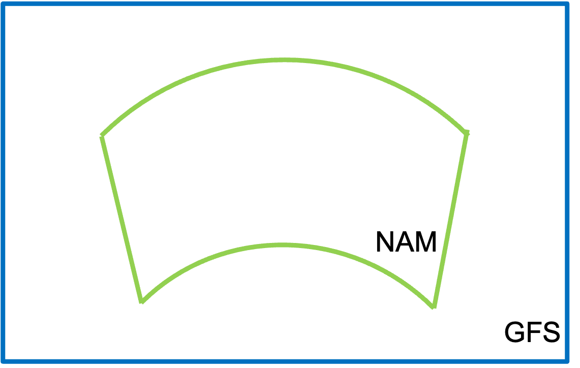
Multiple Data Sources¶

Multiple data sources may be required when a source of meteorological data from a regional model is insufficient to cover the entire simulation domain, and data from a larger regional model, or a global model, must be used when interpolating to the remaining points of the simulation grid.

For example, NAM data is only available over North America. To use NAM data wherever possible, and GFS data elsewhere, both data types will need to be ungribbed.

Process the NAM data

Use the link_grib.csh script to link the NAM data files to the WPS directory.
Link the NAM Vtable to the filename Vtable.
Edit the prefix namelist.wps parameter in the &ungrib record to specify these data. This setting is the user’s choice, and can be a prefix for the ungrib.exe output intermediate files, or can include a path to the files created by ungrib.
```
&ungrib
  out_format = 'WPS',
  prefix = 'NAM',
/
```
Run ungrib.exe, which should produce the following files (with a suitable substitution for the appropriate dates):
```
NAM:2024-08-16_12
NAM:2024-08-16_15
NAM:2024-08-16_18
...
```

Process the GFS data

Use the link_grib.csh script to link the GPS data files to the WPS directory.
Link the GFS Vtable to the filename Vtable.
Change the prefix namelist parameter (in &ungrib) to signify GFS data.
```
&ungrib
  out_format = 'WPS',
  prefix = GFS',
/
```
Run ungrib.exe, which should produce the following output files.
```
GFS:2024-08-16_12
GFS:2024-08-16_15
GFS:2024-08-16_18
...
```
There should now be intermediate files with prefixes of NAM and GFS in the WPS directory.

Run metgrid.exe to interpolate both NAM and GFS data to the domain

To interpolate from multiple sources of time-varying, meteorological data, the fg_name variable in the metgrid namelist record should be set to a list of prefixes of intermediate files, including path information when necessary. When multiple path-prefixes are given, and the same meteorological field is available from more than one of the sources, data from the last-specified source will take priority over all preceding sources. Thus, data sources may be prioritized by the order in which the sources are given.

Note

Because we want to prioritize the NAM data in the location where it is available, it goes last in the list since interpolation goes in order, meaning metgrid processes the GFS data, and then the NAM data, which will overwrite the GFS data where the fields and locations match.

Set the &metgrid namelist record parameter fg_name to the intermediate file prefixes.
```
&metgrid
  fg_name = 'GFS', 'NAM'
/
```
Run metgrid.exe.

Then the resulting model domain would use data as shown in the figure below.

../../_images/wps_nam_gfs_data_domain.png

Using Non-isobaric Meteorological Data Sets¶

When using non-isobaric meteorological data sets to initialize a WRF simulation, they must be supplied to the metgrid.exe program with 3-d pressure and geopotential height fields on the same levels as other 3-d atmospheric variables, such as temperature and humidity. These fields are used by the WRF real.exe pre-processor for vertical interpolation to WRF model levels, for surface pressure computation, and for other purposes.

For some data sources (namely ECMWF model-level data and UK Met Office model data), 3-d pressure and/or geopotential height fields can be derived from the surface pressure and/or surface height fields using an array of coefficients, and the WPS Utility Programs (specifically, calc_ecmwf_p.exe and height_ukmo.exe) are available to perform this derivation.

Other meteorological data sets explicitly provide 3-d pressure and geopotential height fields, and it must only be ensured that these fields exist in the set of intermediate files provided to the metgrid.exe program.

Writing Meteorological Data to the Intermediate Format¶

The ungrib program decodes GRIB data sets into a simple intermediate format required by metgrid. If meteorological data are not available in GRIB format, the user is responsible for writing such data into the intermediate file format. Intermediate format is relatively simple, consisting of a sequence of unformatted Fortran writes. Note that these unformatted writes use big-endian byte order, which can typically be specified with compiler flags. Below, the WPS intermediate format is described.

When writing data to the WPS intermediate format:

2-dimensional fields are written as a rectangular array of real values
3-dimensional arrays must be split across the vertical dimension into 2-dimensional arrays, which are written independently

Note

For global data sets, either a Gaussian or cylindrical equidistant projection must be used, and for regional data sets, either a Mercator, Lambert conformal, polar stereographic, or cylindrical equidistant may be used.

The sequence of writes used to write a single 2-dimensional array is as follows (note that not all variables declared below are used for a given projection of the data).

integer :: version             ! Format version (must =5 for WPS format)
integer :: nx, ny              ! x- and y-dimensions of 2-d array
integer :: iproj               ! Code for projection of data in array:
                               !       0 = cylindrical equidistant
                               !       1 = Mercator
                               !       3 = Lambert conformal conic
                               !       4 = Gaussian (global only!)
                               !       5 = Polar stereographic
real :: nlats                  ! Number of latitudes north of equator
                               !       (for Gaussian grids)
real :: xfcst                  ! Forecast hour of data
real :: xlvl                   ! Vertical level of data in 2-d array
real :: startlat, startlon     ! Lat/lon of point in array indicated by
                               !       startloc string
real :: deltalat, deltalon     ! Grid spacing, degrees
real :: dx, dy                 ! Grid spacing, km
real :: xlonc                  ! Standard longitude of projection
real :: truelat1, truelat2     ! True latitudes of projection
real :: earth_radius           ! Earth radius, km
real, dimension(nx,ny) :: slab ! The 2-d array holding the data
logical :: is_wind_grid_rel    ! Flag indicating whether winds are
                               !       relative to source grid (TRUE) or
                               !       relative to earth (FALSE)
character (len=8)  :: startloc ! Which point in array is given by
                               !       startlat/startlon; set either
                               !       to 'SWCORNER' or 'CENTER  '
character (len=9)  :: field    ! Name of the field
character (len=24) :: hdate    ! Valid date for data YYYY:MM:DD_HH:00:00
character (len=25) :: units    ! Units of data
character (len=32) :: map_source  !  Source model / originating center
character (len=46) :: desc     ! Short description of data

!  1) WRITE FORMAT VERSION
write(unit=ounit) version

!  2) WRITE METADATA
! Cylindrical equidistant
if (iproj == 0) then
        write(unit=ounit) hdate, xfcst, map_source, field, &
                          units, desc, xlvl, nx, ny, iproj
        write(unit=ounit) startloc, startlat, startlon, &
                          deltalat, deltalon, earth_radius

! Mercator
else if (iproj == 1) then
        write(unit=ounit) hdate, xfcst, map_source, field, &
                          units, desc, xlvl, nx, ny, iproj
        write(unit=ounit) startloc, startlat, startlon, dx, dy, &
                          truelat1, earth_radius

! Lambert conformal
else if (iproj == 3) then
        write(unit=ounit) hdate, xfcst, map_source, field, &
                          units, desc, xlvl, nx, ny, iproj
        write(unit=ounit) startloc, startlat, startlon, dx, dy, &
                          xlonc, truelat1, truelat2, earth_radius

                                  ! Gaussian
else if (iproj == 4) then
        write(unit=ounit) hdate, xfcst, map_source, field, &
                          units, desc, xlvl, nx, ny, iproj
        write(unit=ounit) startloc, startlat, startlon, &
                          nlats, deltalon, earth_radius

! Polar stereographic
else if (iproj == 5) then
        write(unit=ounit) hdate, xfcst, map_source, field, &
                          units, desc, xlvl, nx, ny, iproj
write(unit=ounit) startloc, startlat, startlon, dx, dy, &
                          xlonc, truelat1, earth_radius

end if

!  3) WRITE WIND ROTATION FLAG
write(unit=ounit) is_wind_grid_rel

!  4) WRITE 2-D ARRAY OF DATA
write(unit=ounit) slab

WPS Utilities for Data Manipulation¶

The following utilities are available for examining data files, computing pressure fields, and computing average surface temperature fields.

avg_tsfc.exe¶

avg_tsfc.exe

A utility that computes a daily mean surface temperature, given input files in the intermediate format.

avg_tsfc.exe uses data to compute the average, based on the date range and the interval between intermediate files (interval_seconds) specified in the share namelist.wps record.

Note

If a complete day’s worth of data is not available, no output file will be written, and the program will halt. Any intermediate files for dates not used as part of a complete 24-hour period are ignored; for example, if five intermediate files are available at a six-hour interval, the last file is ignored.

The computed average field is written to a new file named TAVGSFC, using the same intermediate format version as the input files. This field is then ingested by metgrid by specifying constants_name = ‘TAVGSFC’ in the metgrid namelist record.

mod_levs.exe¶

mod_levs.exe

A WPS utility that removes levels of data from intermediate format files.

The levels which are to be kept are specified in a new namelist record in the namelist.wps file. For e.g.,

&mod_levs
press_pa = 201300 , 200100 , 100000 ,
            95000 ,  90000 ,
            85000 ,  80000 ,
            75000 ,  70000 ,
            65000 ,  60000 ,
             5000 ,  50000 ,
            45000 ,  40000 ,
            35000 ,  30000 ,
            25000 ,  20000 ,
            15000 ,  10000 ,
             5000 ,   1000
/

press_pa: A &mod_levs namelist variable that specifies a list of levels to keep; these levels should match values of xlvl in the intermediate format files (see Writing Meteorological Data to the Intermediate Format).

mod_levs takes two command-line arguments as its input.

The name of the intermediate file on which to operate
The name of the output file to be written

An example use case for this utility is, for example, when one data set is used for the model initial conditions (ICs) and another is used for the lateral boundary conditions (BCs). This is done by providing the IC data at the initial time to be interpolated by metgrid, and the BC data for all other times. Because real.exe requires a constant number of vertical levels to interpolate from, if both data sets have the same number of vertical levels, then no work needs to be done; however, when they have a different number of levels, it is necessary, at a minimum, to remove (m - n) levels, where m > n and m and n represent the number of levels in each of the two data sets, from the data set with m levels.

Note

Although vertical locations of the levels need not match between data sets, all data sets need surface level data, and, when running real.exe and wrf.exe, the value of p_top_requested must be set to a level below the lowest top among the data sets.

calc_ecmwf_p.exe¶

calc_ecmwf_p.exe

A WPS utility used for ECMWF sigma-level data to place 3D pressure and geopotential height fields on the same levels as all other atmospheric fields, to meet the requirements of the real program for vertical interpolation. Additionally, if soil height (or soil geopotential), 3D temperature, and 3D specific humidity fields are available, calc_ecmwf_p.exe computes a 3D geopotential height field, which is required to obtain an accurate vertical interpolation in the real program.

Given a surface pressure field (or log of surface pressure field) and a list of coefficients (A and B), calc_ecmwf_p.exe computes the pressure at an ECMWF sigma level (k) at grid point (i,j) as Pijk = Ak + Bk*Psfcij. The list of coefficients can be copied from a table appropriate to the number of sigma levels in the data set from one of the following links:

16 Model Level Definitions

L19 Model Level Definitions

L31 Model Level Definitions

L40 Model Level Definitions

L50 Model Level Definitions

L60 Model Level Definitions

L62 Model Level Definitions

L91 Model Level Definitions

L137 Model Level Definitions

This table should be written in plain text to a new file (ecmwf_coeffs) in the working directory; for example, with 16 sigma levels, ecmwf_coeffs would contain:

       0.000000      0.000000000
    5000.000000      0.000000000
    9890.519531      0.001720764
   14166.304688      0.013197623
   17346.066406      0.042217135
   19121.152344      0.093761623
   19371.250000      0.169571340
   18164.472656      0.268015683
   15742.183594      0.384274483
   12488.050781      0.510830879
   8881.824219      0.638268471
   5437.539063      0.756384850
   2626.257813      0.855612755
    783.296631      0.928746223
      0.000000      0.972985268
      0.000000      0.992281914
      0.000000      1.000000000

When computing a 3D geopotential height field, soil height (or soil geopotential), 3-d temperature, and 3-d specific humidity must be available.

Using the intermediate files produced by ungrib and the file ecmwf_coeffs, calc_ecmwf_p.exe loops over all time periods in namelist.wps, and produces an additional intermediate file, PRES:YYYY-MM-DD_HH, for each time. Each PRES file contains pressure and geopotential height for each full sigma level, as well as a 3D relative humidity field.

Before running metgrid, set fg_name to the prefixes for both the intermediate data produced by ungrib, and the new PRES data.

fg_name = 'FILE','PRES'

height_ukmo.exe¶

calc_ecmwf_p.exe

A WPS utility that computes a geopotential height field, which is absent from UKMO Unified Model data, but is required by the real program for vertical interpolation.

The height_ukmo.exe program computes 3D geopotential height using the SOILHGT field (from the intermediate files created by ungrib), with the aid of an auxiliary table. The computed height field is written to a new intermediate file with the prefix HGT, which is then be added to the fg_name namelist variable in the &metgrid namelist record before running metgrid.exe. For e.g.,

&metgrid
 fg_name = 'FILE','HGT'

The name of the file containing the auxiliary table is hard-wired in the height_ukmo.exe code, but the name must be changed in WPS/util/src/height_ukmo.F to the name of the table with the same number of levels as the GRIB data processed by ungrib.exe. The following tables are provided in the WPS/util directory:

vertical_grid_38_20m_G3.txt : for data with 38 levels
vertical_grid_50_20m_63km.txt : for data with 50 levels
vertical_grid_70_20m_80km.txt : for data with 70 levels

g1print.exe and g2print.exe¶

g1print.exe

A WPS utility that prints a listing of fields, levels, and dates in a GRIB Edition 1 file

g2print.exe

A WPS utility that prints a listing of fields, levels, and dates in a GRIB Edition 2 file

These programs take as their only command-line argument the name of a GRIB Edition 1 or 2 file. To run these programs, from the WPS directory, type

> ./util/g1print.exe path-to-gribbed-file>/<grib1_file

where path-to-gribbed-file and grib1_file should be replaced with the path and file name.

The same syntax is used for the g2print.exe program, as well.

rd_intermediate.exe¶

rd_intermediate.exe

A WPS utility that prints information about the fields contained in an ungrib-produced intermediate file

To run this program, from the WPS directory, type

> ./util/rd_intermediate.exe PREFIX:YYYY-MM-DD_hh

where PREFIX:YYYY-MM-DD_hh should be replaced with the intermediate file name.

The Metgrid Program¶

The metgrid program is responsible for the following functions:

Horizontally interpolating meteorological data (extracted by ungrib) to simulation domains (defined by geogrid)
Rotating winds to the WRF grid - i.e., rotating so that the U-component is parallel to the x-axis and the V-component is parallel to the y-axis

KKW - COME GET THESE 2 PARAGRAPHS FOR OTHER SECTIONS The METGRID.TBL file controls how each meteorological field is interpolated. It provides one section for each field, and within a section, it is possible to specify options such as interpolation methods to be used for the field, the field that acts as the mask for masked interpolations, and the grid staggering (e.g., U, V) to which a field is interpolated.

Output from metgrid is written in the WRF I/O API format, and thus, by selecting the netCDF I/O format, metgrid can be made to write its output in netCDF for easy visualization using external software packages, including the new version of RIP4.

Masked Interpolation¶

Masked Fields

Meteorological data that have missing values for some grids, or may only have valid data for a subset of the grid points

During horizontal interpolation, the metgrid program must process masked fields differently than unmasked data. For e.g., the sea surface temperature (SST) field often only has valid values for the grid points over water. There are two different ways metgrid can determine which points are invalid (masked):

If the gridded dataset comes with a separate field that identifies land and water points (LANDSEA)
Every field uses a special missing value to identify invalid points for that field

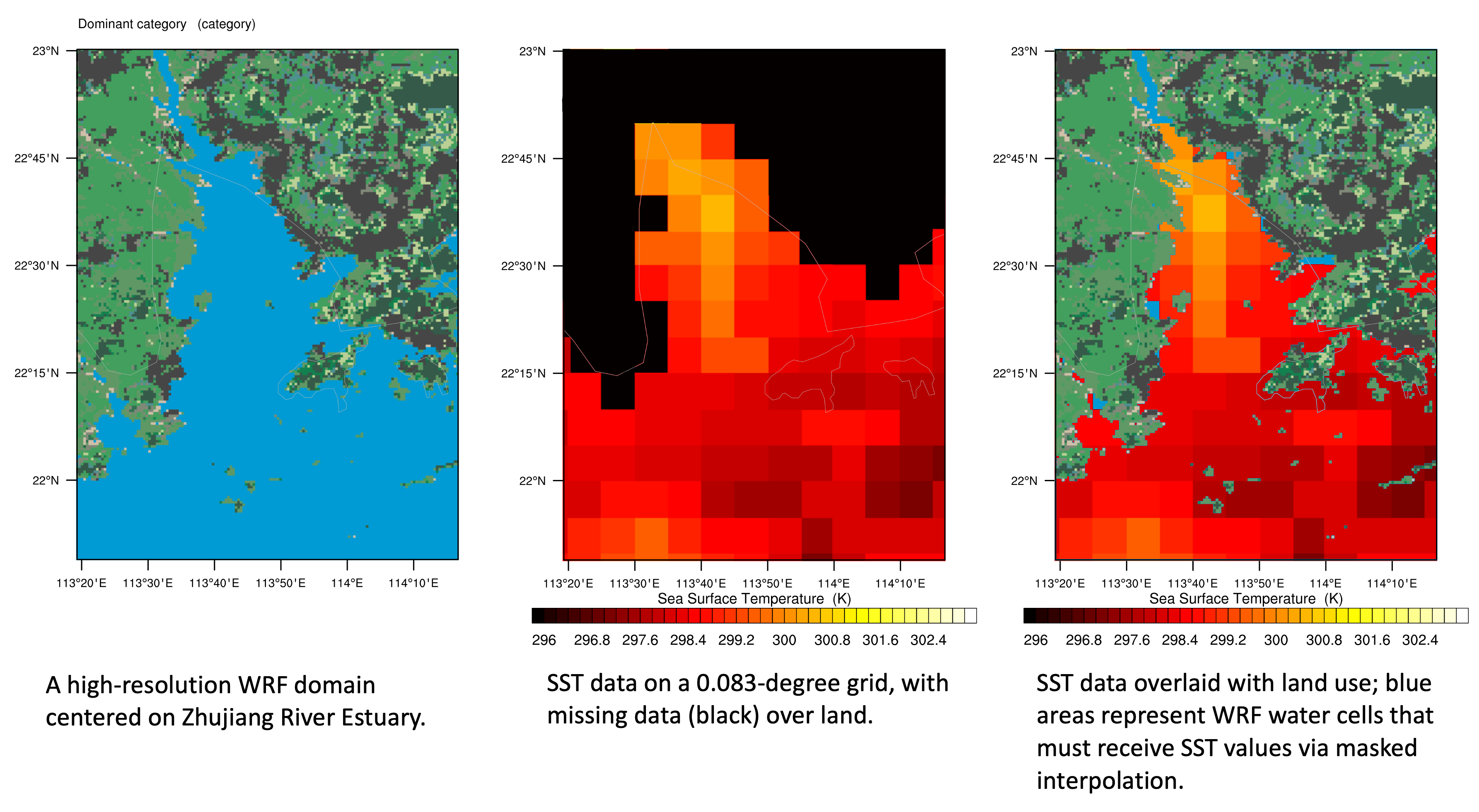
The below image shows an example of how masked interpolation works. The figure on the left shows a plot of the landuse index field for the WRF domain, where the water points are all blue. The center panel shows SST data, available at a coarser resolution than that of the model domain, meaning there are water points in the model domain that are not covered by the SST data set, and there are some land points that are covered by the SST data set. The panel on the right shows SST data overlaid with the domain’s landuse. Any of the remaining blue areas near the coast represent WRF water cells for which metgrid must perform masked interpolation.

Wind Vector Rotation¶

During horizontal interpolation, metgrid interpolates meteorological fields to their proper staggering in the WRF model grid:

The U-component is interpolated directly to the u-staggerd points in each grid cell.
The V-component is interpolated directly to the v-staggerd points in each grid cell.
All other scalar value fields are interpolated directly to the mass centers of each grid cell.

Input wind fields (U-component + V-component) are either

Earth-relative
The U-component = the westerly component and the V-component = the southerly component
Relative to the source grid
The U-component is parallel to the source model’s x-axis and the V-component is parallel to the source model’s y-axis

The WRF model expects wind components relative to the simulation grid. Because the WRF domains are laid out on a specific map projection, the westerly component, for e.g., is not always the same as the x-component, and the southerly component is not always the same as the y-component. Therefore, metgrid must rotate the wind field so that its components are with respect to the model’s x and y directions.

METGRID.TBL¶

METGRID.TBL

A text file that defines parameters of each meteorological field to be interpolated by metgrid.

Each field’s parameters are defined in a separate section, where sections are delimited by a line of equality symbols (e.g., ‘==============’). Within each section are specifications, each using the form keyword=value. Some keywords are required, while others are optional; some keywords are mutually exclusive with other keywords. Each possible keyword and its expected range of values are described in the table below.

Variable Name	Default Value	Description
name	no default	A character string representing the name of the meteorological field to which the containing section of the table pertains. The name should be identical to the field’s name in the intermediate files (and in the Vtable used) This field is required.
output	yes	Either yes or no, indicating whether the field is to be written to the metgrid output files
mandatory	no	Either yes or no, indicating whether the field is required for successful completion of metgrid
output_name	no default	A character string giving the name the interpolated field should be output as. When a value is specified, the interpolation options from the field’s table section are used.
from_input	no default	A character string compared against the values in the fg_name namelist variable; if from_input is specified, the containing table section is only used if the time-varying input source has a filename that contains the value of from_input as a substring. This may be used to specify different interpolation options for the same field, depending on which source of the field is being processed
output_stagger	M	The model grid staggering to which the field should be interpolated; this must be one of U, V, and M
is_u_field	no	Either yes or no, indicating whether the field should be used as the U-component wind field; the U-component wind field must be interpolated to the U staggering (output_stagger=U)
is_v_field	no	Either yes or no, indicating whether the field should be used as the V-component wind field; the V-component wind field must be interpolated to the V staggering (output_stagger=V)
interp_option	nearest_neighbor	A sequence of one or more character strings representing the names of interpolation methods to be used when horizontally interpolating the field. Available interpolation methods are: average_4pt, average_16pt, wt_average_4pt, wt_average_16pt, nearest_neighbor, four_pt, sixteen_pt, search(r), and average_gcell(r). For the search method, the optional argument r specifies the maximum search radius in units of source data grid points (with a default of 1200 points. For average_gcell, the optional argument r specifies the minimum ratio of source data resolution to simulation grid resolution at which the method will be applied; unless specified, r = 0.0, and the option is used for any ratio. When a sequence of two or more methods are given, the methods should be separated by a + sign
interp_mask	no mask	The name of the field to be used as an interpolation mask, along with the value within that field that signals masked points and an optional relational symbol, < or >. A specification takes the form field(?maskval), where field is the name of the field, ? is an optional relational symbol (< or >), and maskval is a real value. Source data points are not used in interpolation if the corresponding point in the field is equal, greater than, or less than the value of maskval for no relational symbol, a > symbol, or a < symbol, respectively
interp_land_mask	no mask	The name of the field to be used as an interpolation mask when interpolating to water points (determined by the static LANDMASK field), along with the value within that field that signals land points and an optional relational symbol, < or >. A specification takes the form field(?maskval), where field is the name of the field, ? is an optional relational symbol (< or >), and maskval is a real value
interp_water_mask	no mask	The name of the field to be used as an interpolation mask when interpolating to land points (determined by the static LANDMASK field), along with the value within that field that signals water points and an optional relational symbol, < or >. A specification takes the form field(?maskval), where field is the name of the field, ? is an optional relational symbol (< or >), and maskval is a real value
fill_missing	1.00E+20	A real number specifying the value to be assigned to model grid points that received no interpolated value, for example, because of missing or incomplete meteorological data
z_dim_name	num_metgrid_levels	For 3-dimensional meteorological fields, a character string giving the name of the vertical dimension to be used for the field on output
derived	no	Either yes or no, indicating whether the field should be derived from other interpolated fields, rather than interpolated from an input field
fill_lev	no default	If a field has a missing level, fill_lev specifies how the level should be filled. fill_lev may be used multiple times within a table section. A generic value takes the form DLEVEL:FIELD(SLEVEL), where DLEVEL : specifies the level to be filled (either an integer or the string all) FIELD : specifies the source field from which to copy levels (either the name of another field, the string const, or the string vertical_index) SLEVEL : specifies the level to use - If FIELD is specified as const, then SLEVEL is a constant value that will be used to fill with; if FIELD is specified as vertical_index, SLEVEL must not be specified, and the value of the vertical index of the source field is used; if DLEVEL is all, then all levels from the field specified by the level_template keyword are used to fill the corresponding levels in the field, one at a time
level_template	no default	A character string giving the name of a field from which a list of vertical levels should be obtained and used as a template. This keyword is used in conjunction with a fill_lev specification that uses all in the DLEVEL part of its specification
masked	<null> (i.e., the field is valid for both land and water points, Either land, water, or both	If set to land or water the field is not interpolated to WRF land or water points, respectively; if set to both, the field is interpolated to WRF land points using only land points and water points in the source data. When a field is masked, or invalid, the static LANDMASK field is used to determine which model grid points the field should be interpolated to; invalid points are assigned the value of the FILL_MISSING keyword. Whether a source data point is land or water is determined by the masks specified using the INTERP_LAND_MASK and INTERP_WATER_MASK options
missing_value	no default	A real number giving the value in the input field that is assumed to represent missing data
vertical_interp_option	no default	A character string specifying the vertical interpolation method to use when vertically interpolating to missing points. Currently, this option is not implemented
flag_in_output	<null> (i.e., no flag will be written for the field)	A character string giving the name of a global attribute that will be assigned a value of 1 and written to metgrid output if the interpolated field is to be output (output=yes)

When metgrid is run, it looks for a table with the name “METGRID.TBL.” By default, this table is linked to METGRID.TBL.ARW, as is shown below. To use a different table, link that table to the expected name METGRID.TBL.

> ls -ls metgrid/METGRID.TBL

  lrwxrwxrwx  1         15  METGRID.TBL -> METGRID.TBL.ARW

Running the WPS¶

There are three primary steps to running the WRF Preprocessing System.

Run geogrid to define the model domain, and to interpolate static fields to each model grid point
Run ungrib to extract meteorological fields from GRIB data sets for the simulation period
Run metgrid to horizontally interpolate meteorological fields to the model domains

Note

When running multiple simulations for the same model domain, geogrid only needs to be run once; thereafter, only time-varying data need to be processed for each simulation using ungrib and metgrid. Similarly, if several model domains are being run for the same time period using the same meteorological data source, it is not necessary to run ungrib separately for each simulation.

If the WPS software was successfully installed, symbolic links to the geogrid.exe, ungrib.exe, and metgrid.exe programs should exist from the root of the WPS directory structure. A listing in the WPS root directory should look something like:

> ls -ls

drwxr-xr-x 2   4096 arch
-rwxr-xr-x 1   1765 clean
-rwxr-xr-x 1   4795 compile
-rw-r--r-- 1 118862 compile.log
-rwxr-xr-x 1  16613 configure
-rw-r--r-- 1   3424 configure.wps
drwxr-xr-x 4   4096 geogrid
lrwxrwxrwx 1     23 geogrid.exe -> geogrid/src/geogrid.exe
-rwxr-xr-x 1   1331 link_grib.csh
drwxr-xr-x 3   4096 metgrid
lrwxrwxrwx 1     23 metgrid.exe -> metgrid/src/metgrid.exe
-rw-r--r-- 1    705 namelist.wps
-rw-r--r-- 1   2749 namelist.wps.all_options
-rw-r--r-- 1   1637 namelist.wps.global
-rw-r--r-- 1   6232 README
drwxr-xr-x 4   4096 ungrib
lrwxrwxrwx 1     21 ungrib.exe -> ungrib/src/ungrib.exe
drwxr-xr-x 3   4096 util

Run the Geogrid Program¶

The following steps are required to run the geogrid program (assumming Geographic Static Fields have already been obtained):

Modify namelist.wps for variables specific to the geogrid program
Run the geogrid executable (geogrid.exe)

1. Modify namelist.wps for Geogrid¶

Prior to running geogrid, namelist.wps must be configured to define the model coarse domain and any nested domains. This requires modifications to the &geogrid and &share namelist records, as those are the records the geogrid program reads.

Note

See WPS Namelist Variables for detailed descriptions of all namelist.wps variables.

&geogrid

Below is an example of the &geogrid namelist record, followed by descriptions of the variables.

&geogrid
  parent_id         =   1,   1,
  parent_grid_ratio =   1,   3,
  i_parent_start    =   1,  53,
  j_parent_start    =   1,  25,
  e_we              =  150, 220,
  e_sn              =  130, 214,
  geog_data_res     = 'default','default',
  dx = 15000,
  dy = 15000,
  map_proj = 'lambert',
  ref_lat   =  33.00,
  ref_lon   = -79.00,
  truelat1  =  30.0,
  truelat2  =  60.0,
  stand_lon = -79.0.,
  geog_data_path = '/glade/work/wrfhelp/WPS_GEOG/'
/

The following &geogrid namelist parameters are specific to the Geographic Static Fields.

geog_data_res	The resolution(s) to be used when interpolating static data to the domain’s grid
geog_data_path	The path to the directory where static field files are located; the value should match one of the data resolutions in the GEOGRID.TBL

The following &geogrid namelist parameters are specific to the Map Projection and the location of the domain on the earth.

map_proj	The map projection to be used for the simulation domain; accepted projections are ‘lambert’, ‘polar’, ‘mercator’, and ‘lat-lon’
truelat1 truelat2	The latitude(s) at which the surface of projection intersects or is tangent to the surface of the earth; only the lambert projection requires a setting for truelat2
ref_lat ref_lon	The latitude and longitude location whose (i,j) location is known; the default values are the latitude,longitude of the center point of the coarse domain; these variables do not apply to global simulations
pole_lat pole_lon	The latitude and longitude of the geographic north pole within the model’s computational grid; these parameters are only used for a lat-lon projection
stand_lon	Specifies the meridian parallel to the y-axis

The following &geogrid namelist parameters are specific to the simulation domain’s resolution and size. See The Computational Grid for details.

e_we e_sn	The number of velocity points (computed along the edges of grid cells) in the west-east and south-north directions, respectively, for each domain, determining each domain’s full dimensions
dx / dy	The nominal grid distance where map factor=1 in the x and y directions; this is computed in degrees for the rotated lat-lon map projection, but is computed in meters for all other projections; these variables do not apply to global simulations

The following &geogrid namelist parameters are specific to Nested Domains.

parent_id	Specifies the parent of each nested child. Every nest must be a child of exactly one other domain, with the coarse domain being its own parent
parent_grid_ratio	Specifies the nest’s refinement ratio with respect to its parent, determining the nominal grid spacing for a nest in relation to the grid spacing of the its parent
i_parent_start j_parent_start	Indicates the (i,j) lower left corner of a nest - specifically the (i,j) point where this corner is inside its parent. The specified location is given with respect to the unstaggered grid.

&share

In addition to the &geogrid namelist modifications, a few additional settings are required in the &share record - an example of which is shown below, followed by descriptions of the geogrid-relevant parameters.

&share
  wrf_core = 'ARW',
  max_dom = 2,
  start_date = '2019-09-04_12:00:00','2019-09-04_12:00:00',
  end_date   = '2019-09-06_18:00:00','2019-09-04_12:00:00',
  interval_seconds = 10800,
  io_form_geogrid = 2
/

wrf_core	Specifies which WRF dynamical core is being used. Set to ‘ARW’ for a WRF-ARW simulation
max_dom	The total number of domains; for a single domain simulation, this is set to “1”
io_form_geogrid	The output format for geogrid-produced files (geo_em*); the default is 2 (netCDF).

Since geogrid produces only time-independent data, the start_date, end_date, and interval_seconds variables are ignored by geogrid.

Note

An optional variable, opt_output_from_geogrid_path, may be set in the &share section to place geogrid output files in a location other than the default location (the top-level WPS directory).

2. Run geogrid.exe¶

Having suitably defined the simulation domain(s) in namelist.wps, the geogrid executable (geogrid.exe) may be run to produce domain files. Issue the following command in the WPS directory.

> ./geogrid.exe

When geogrid.exe has finished running, the following message should be printed to the screen, and to a new geogrid.log created in the top-level WPS directory.

!!!!!!!!!!!!!!!!!!!!!!!!!!!!!!!!!!!!!!!!!!!!!
!  Successful completion of geogrid.        !
!!!!!!!!!!!!!!!!!!!!!!!!!!!!!!!!!!!!!!!!!!!!!

A listing of the WPS root directory (or the directory specified by opt_output_from_geogrid_path, if this variable was set) should display the domain files. If not, consult the geogrid.log file to determine the possible cause of failure. See Checking WPS Output for more information.

> ls -ls

-rw-r--r-- 1  1957004 geo_em.d01.nc
-rw-r--r-- 1  4745324 geo_em.d02.nc
-rw-r--r-- 1    11169 geogrid.log

Domain files are named geo_em.d0N.nc, where N is the number of the nest defined in each file. The file suffix will vary depending on the io_form_geogrid setting in namelist.wps.

Run the Ungrib Program¶

Assuming GRIB-formatted meteorological data (see Required Input for Running WRF) have been downloaded, the following steps are required to run the ungrib program:

Modify namelist.wps for variables specific to the ungrib program
Link the meteorological data to the WPS directory
Link the correct Vtable to the WPS directory
Run the ungrib executable (ungrib.exe)

1. Modify namelist.wps for Ungrib¶

Prior to running ungrib, namelist.wps must be configured for ungrib. This requires modifications to the &ungrib and &share namelist records, as those are the records the ungrib program reads.

&ungrib

Below is an example of the &ungrib namelist record, followed by variable descriptions.

&ungrib
  out_format = 'WPS',
  prefix     = 'FILE'
/

out_format	Specifies the intermediate data format; keep this set to ‘WPS’
prefix	The prefix to be appended to the intermediate files; e.g., if prefix is set to ‘GFS’, intermediate files are named GFS:YYYY-MM-DD_HH, where YYYY-MM-DD_HH is the valid time of the data in the file; a path that includes the prefix may be used, if desired

&share

Below is an example of the &share namelist record, followed by variable descriptions.

&share
  wrf_core = 'ARW',
  max_dom = 2,
  start_date = '2019-09-04_12:00:00','2019-09-04_12:00:00',
  end_date   = '2019-09-04_18:00:00','2019-09-04_12:00:00',
  interval_seconds = 10800,
  io_form_geogrid = 2
/

The following share namelist variables are relevant to ungrib

start_date end_date	the starting and ending times of the coarse domain; ungrib is not domain-dependent, so it does not look at settings for nests, but values for nests do not need to be removed
interval_seconds	the interval (in seconds) between meteorological data files

2. Link-in Meteorological Data¶

Ungrib attempts to read GRIB files named GRIBFILE.AAA, GRIBFILE.AAB, …, GRIBFILE.ZZZ. To link the meteorological input GRIB files to these filenames, a shell script, link_grib.csh, is provided in the top-level WPS directory. The script takes as a command-line argument a list of GRIB files to be linked. For example, if the GRIB data were downloaded to the directory /data/gfs, the files are linked as follows:

> ls -ls /data/gfs

-rw-r--r-- 1  42728372 gfs_20190904_12_00
-rw-r--r-- 1  48218303 gfs_20190904_12_03
-rw-r--r-- 1  48218303 gfs_20190904_12_06


> ./link_grib.csh /data/gfs/gfs*

Note

Notice in the above command, there is no “.” after the command, which would indicate to put the files “here.” This is built into the script, so there is no need to issue any command after the file prefix.

After running this command, there should be a GRIBFILE.XXX file available for each GFS file. In the above example, there are three files available, so a file listing in the WPS directory should reveal the following files:

> ls -ls

-rw-r--r--  1  29 GRIBFILE.AAA -> /data/gfs/gfs_20190904_12_00
-rw-r--r--  1  29 GRIBFILE.AAB -> /data/gfs/gfs_20190904_12_03
-rw-r--r--  1  29 GRIBFILE.AAC -> /data/gfs/gfs_20190904_12_06

3. Link to the Correct Vtable¶

Prior to running the ungrib program, a Vtable containing the GRIB codes for the type of input data being used must be linked to the top-level WPS directory. When ungrib runs, it looks for a file with the generic name “Vtable” in the running directory. Vtable.* files are available for many sources of meteorological data in the /ungrib/Variable_Tables directory. The appropriate Vtable should be symbolically linked to the file Vtable. For example, if the GRIB data are from the GFS model:

> ln -s ungrib/Variable_Tables/Vtable.GFS Vtable

4. Run ungrib.exe¶

After the above three steps are complete, the ungrib executable (ungrib.exe) is run to produce meteorological data files in the intermediate format. To run ungrib, type the following:

> ./ungrib.exe

If ungrib.exe runs successfully, the following message will be printed to the screen, and to the ungrib.log file created during ungrib’s execution.

!!!!!!!!!!!!!!!!!!!!!!!!!!!!!!!!!!!!!!!!!!!!!
!  Successful completion of ungrib.         !
!!!!!!!!!!!!!!!!!!!!!!!!!!!!!!!!!!!!!!!!!!!!!

If ungrib was successful, the intermediate files should be available in the current working directory. Intermediate files written by ungrib will have names of the form FILE:YYYY-MM-DD_HH (unless the prefix variable was set to a prefix other than FILE in the &ungrib section of the namelist).

> ls -ls

-rw-r--r-- 1  154946888 FILE:2019-09-04_12
-rw-r--r-- 1  154946888 FILE:2019-09-04_15
-rw-r--r-- 1  154946888 FILE:2019-09-04_18

Run the Metgrid Program¶

The following steps are required to run the metgrid program:

Modify namelist.wps for variables specific to the metgrid program
Run the metgrid executable (metgrid.exe)

1. Modify namelist.wps for Metgrid¶

In the final step of running the WPS, meteorological data extracted by ungrib are horizontally interpolated to the simulation grids defined by geogrid. Prior to running metgrid, namelist.wps must be configured for metgrid. This requires modifications to the &metgrid and &share namelist records, as those are the records the metgrid program reads.

&metgrid

Below is an example of the &metgrid namelist record, followed by variable descriptions.

&metgrid
  fg_name                      = 'FILE',
  io_form_metgrid              = 2,
/

fg_name	The prefix of the intermediate files; this usually matches the setting for prefix in the &ungrib namelist record; a path that includes the prefix may be used, if desired
io_form_metgrid	the output format for the horizontally interpolated files; the default (2) indicates files will be in netCDF format

Note

Optional variables may be set in the &metgrid namelist record:

opt_output_from_metgrid_path - to write metgrid output to a location other than the default location - the top-level WPS directory
opt_metgrid_tbl_path - to set a location for the metgrid program to find the METGRID.TBL if it is in any location other than the default - in the WPS/metgrid directory
constants_name - to set the file names of any intermediate files containing constant fields; a path that includes the file name may be used, if desired; see Interpolating Time-invariant Fields for details

&share

Below is an example of the &share namelist record.

&share
  wrf_core = 'ARW',
  max_dom = 2,
  start_date = '2019-09-04_12:00:00','2019-09-04_12:00:00',
  end_date   = '2019-09-04_18:00:00','2019-09-04_12:00:00',
  interval_seconds = 10800,
  io_form_geogrid = 2
/

By this point, there is generally no need to change any variables in the &share namelist record, since those variables should have been suitably set in previous steps. If the share namelist was not edited while running geogrid and ungrib, however, the following parameters must be set before running metgrid (see Run the Geogrid Program and Run the Ungrib Program for descriptions of these variables).

wrf_core
max_dom
start_date, end_date
interval_seconds

2. Run metgrid.exe¶

After editing namelist.wps, metgrid is run by issuing the command

> ./metgrid.exe

If metgrid successfully ran, the following message should print to the screen, and to the metgrid.log created during processing.

!!!!!!!!!!!!!!!!!!!!!!!!!!!!!!!!!!!!!!!!!!!!!
!  Successful completion of metgrid.        !
!!!!!!!!!!!!!!!!!!!!!!!!!!!!!!!!!!!!!!!!!!!!!

Metgrid output files should now be available in the WPS root directory (or in the directory specified by opt_output_from_metgrid_path, if this variable was set). These files are named met_em.d0N.YYYY-MM-DD_HH:mm:ss.nc, where N is the number of the nest whose data reside in the file. Here, YYYY-MM-DD_HH:mm:ss refers to the date of the interpolated data in each file. If these files do not exist for each of the times in the range given in the share namelist record, consult the metgrid.log file to determine the problem in running metgrid.

> ls -ls

-rw-r--r-- 1    5217648 met_em.d01.2008-03-24_12:00:00.nc
-rw-r--r-- 1    5217648 met_em.d01.2008-03-24_18:00:00.nc
-rw-r--r-- 1   12658200 met_em.d02.2008-03-24_12:00:00.nc
-rw-r--r-- 1      65970 metgrid.log

Once the metgrid output files are created, the WPS process is complete and the real.exe and then wrf.exe programs can be run.

Interpolating Time-invariant Fields¶

The metgrid program is capable of interpolating time-invariant fields using the constants_name variable in the &metgrid namelist record. This variable may be set to a list of filenames - including path information where necessary - of intermediate-formatted files that contain time-invariant fields, to be used in the output for every time period processed by metgrid. For example, short simulations may use a constant SST field; this field need only be available at a single time, and may be used by setting constants_name as follows:

&metgrid
  constants_name = '/data/ungribbed/constants/SST_FILE:2006-08-16_12'
/

or

&metgrid
  constants_name = 'LANDSEA', 'SOILHGT'
/

Parallelism in the WPS¶

If model domain dimensions are too large to fit in a single CPU’s memory, the geogrid and metgrid programs can be run in a distributed memory configuration. To compile geogrid and metgrid for distributed memory execution, MPI libraries must be installed on the target machine, and WPS must be compiled using one of the “DM parallel” configuration options (See the chapter on Compiling for a complete description of compiling the WPS). The geogrid and metgrid programs may then be run with the mpirun or mpiexec commands, or through a batch queuing system, depending on the machine.

The ungrib program is not amenable to parallelization, and the memory requirements for ungrib’s processing are independent of those for geogrid and metgrid; thus, ungrib is always compiled for a single processor and run on a single CPU, regardless of the configuration option selected.

Each of the standard WRF I/O API formats (netCDF, GRIB1, binary) has a corresponding parallel format, whose number is given by adding 100 to the io_form value (i.e., the value of io_form_geogrid and io_form_metgrid) for the standard format. It is not necessary to use a parallel io_form, but when one is used, each CPU reads/writes its input/output to a separate file, whose name is the name that would be used during serial execution, but with a four-digit processor ID appended to the name. For example, running geogrid on four processors with io_form_geogrid=102 creates output files named geo_em.d01.nc.0000, geo_em.d01.nc.0001, geo_em.d01.nc.0002, and geo_em.d01.nc.0003 for the coarse domain.

During distributed-memory execution, model domains are decomposed into rectangular patches, with each processor working on a single patch. When reading/writing from/to the WRF I/O API format, each processor only reads/writes its own patch. If a parallel io_form is chosen for geogrid output, metgrid must be run using the same number of processors as were used to run geogrid. Similarly, if a parallel io_form is chosen for metgrid output, the real program must be run using the same number of processors. It is also possible to use a standard io_form when running on multiple processors, in which case all data for the model domain is distributed/collected upon input/output. When geogrid or metgrid are run on multiple processors, each processor writes its own log file with names appended with the same four-digit processor ID numbers used for the I/O API files.

WPS Namelist Variables¶

&share Record¶

This section describes variables used by more than one WPS program. For example, max_dom specifies the number of domain (the parent, and nests, if applicable) to process - information needed by both the geogrid and metgrid programs.

Variable Name	Default Value	Description
wrf_core	ARW	A character string (either ARW or NMM) that tells the WPS for which dynamical core the input data are being prepared
max_dom	1	An integer specifying the total number of domains (parent domain, plus any nests) used in the simulation
start_year	no default	A list of 4-digit integers specifying the starting UTC year of the simulation for each domain
start_month	no default	A list of 2-digit integers specifying the starting UTC month of the simulation for each domain
start_day	no default	A list of 2-digit integers specifying the starting UTC day of the simulation for each domain
start_hour	no default	A list of 2-digit integers specifying the starting UTC hour of the simulation for each domain
end_year	no default	A list of 4-digit integers specifying the ending UTC year of the simulation for each domain
end_month	no default	A list of 2-digit integers specifying the ending UTC month of the simulation for each domain
end_day	no default	A list of 2-digit integers specifying the ending UTC day of the simulation for each domain
end_hour	no default	A list of 2-digit integers specifying the ending UTC hour of the simulation for each nest
start_date	no default	A list of character strings of the form YYYY-MM-DD_HH:mm:ss specifying the starting UTC date of the simulation for each domain; this variable is an alternate to specifying start_year, start_month, start_day, and start_hour; if both methods are used, the start_date takes precedence
end_date	no default	A list of character strings of the form YYYY-MM-DD_HH:mm:ss specifying the ending UTC date of the simulation for each domain; this variable is an alternate to specifying end_year, end_month, end_day, and end_hour; if both methods are used, the end_date takes precedence
interval_seconds	no default	The integer number of seconds between time-varying meteorological input files
active_grid	true	A list of logical values specifying, for each grid, whether that grid should be processed by geogrid and metgrid
io_form_geogrid	2 (netCDF)	The WRF I/O API format in which geogrid output will be written; possible options are: 1 - binary; output suffix - .int 2 - netCDF; output suffix - .nc 3 - GRIB1; output suffix - .gr1
output_from_geogrid	current working directory (i.e., ./ )	A character string giving the relative or absolute path to the location where geogrid output should be written to and read from
debug_level	0	An integer indicating the extent to which different types of messages should be sent to standard output; when debug_level=0, only generally useful messages and warning messages are written to standard output; when debug_level > 100, additional messages that provide further runtime details are written to standard output; debugging messages and messages specifically intended for log files are never written to standard output, but are always written to the log files; NOTE: setting debug_level > 0 is not typically recommended, as it rarely provides useful information and adds a lot of junk to standard output, creating large, unreadable files

&geogrid Record¶

This section includes variables specific to the geogrid program. These variables primarily define the size and location of all model domains, and where the static geographical data are found.

Variable Name	Default Value	Description
parent_id	1	A list of integers specifying, for each nest, the domain number of the nest’s parent; for the coarsest domain should be set to 1
parent_grid_ratio	no default	A list of integers specifying, for each nest, the nesting ratio relative to the domain’s parent
i_parent_start	no default	A list of integers specifying, for each nest, the x-coordinate of the lower-left corner of the nest in the parent’s unstaggered grid; the coarsest domain should be set to 1
j_parent_start	no default	A list of integers specifying, for each nest, the y-coordinate of the lower-left corner of the nest in the parent’s unstaggered grid; the coarsest domain should be set to 1
s_we	1	A list of integers that should all be set to 1; this variable is optional
e_we	no default	A list of integers specifying, for each nest, the nest’s full west-east dimension; for nested domains, e_we must be one greater than an integer multiple of the nest’s parent_grid_ratio (i.e., e_we = n*parent_grid_ratio+1 for some positive integer n)
s_sn	1	A list of integers that should all be set to 1; this variable is optional
e_sn	no default	A list of integers specifying, for each nest, the nest’s full south-north dimension; for nested domains, e_sn must be one greater than an integer multiple of the nest’s parent_grid_ratio (i.e., e_sn = n*parent_grid_ratio+1 for some positive integer n)
geog_data_res	‘default’	A list of character strings specifying, for each nest, which resolution is used for each static terrestrial field when being interpolated to the grid; a list of resolutions may also be specified - if so, they should be separated by + symbols; the GEOGRID.TBL lists each possible field, along with resolutions displayed preceding a colon in a rel_path or abs_path specification - geog_data_res settings should contain an existing resolution from the GEOGRID.TBL; if not, a default data resolution for that field (if one is specified) is used; if multiple resolutions match, the first match encountered in namelist.wps is used
dx dy	no default	A real value specifying the grid distance in the x-direction and y-direction where the map scale factor is 1; the grid distance is in meters for the ‘polar’, ‘lambert’, and ‘mercator’ projections, and in degrees longitude for the ‘lat-lon’ projection; grid distances for nests are determined recursively based on values specified for parent_grid_ratio and parent_id
map_proj	lambert	A character string specifying the projection of the simulation domain; accepted projections are ‘lambert’, ‘polar’, ‘mercator’, and ‘lat-lon’
ref_lat	no default	A real value specifying the latitude part of a (latitude, longitude) location whose (i,j) location in the simulation domain is known; by default, this value is the latitude of the coarse domain’s center-point
ref_lon	no default	A real value specifying the longitude part of a (latitude, longitude) location whose (i, j) location in the simulation domain is known; by default, this value is the longitude of the coarse domain’s center-point
ref_x	(((E_WE-1.)+1.)/2.) = (E_WE/2.)	A real value specifying the i part of an (i, j) location whose (latitude, longitude) location in the simulation domain is known; the (i, j) location is always given with respect to the mass-staggered grid, whose dimensions are one less than the dimensions of the unstaggered grid
ref_y	(((E_SN-1.)+1.)/2.) = (E_SN/2.)	A real value specifying the j part of an (i, j) location whose (latitude, longitude) location in the simulation domain is known; the (i, j) location is always given with respect to the mass-staggered grid, whose dimensions are one less than the dimensions of the unstaggered grid
truelat1	no default	A real value specifying the first true latitude for the Lambert conformal projection, or the only true latitude for the Mercator and polar stereographic projections
truelat2	no default	A real value specifying the second true latitude for the Lambert conformal conic projection; for all other projections, truelat2 is ignored
stand_lon	no default	A real value specifying the longitude that is parallel with the y-axis in the Lambert conformal and polar stereographic projections; for the regular latitude-longitude projection, this value gives the rotation about the earth’s geographic poles
pole_lat	90	For the latitude-longitude projection, the latitude of the North Pole with respect to the computational latitude-longitude grid in which -90.0 degrees latitude is at the bottom of a global domain, 90.0 degrees latitude is at the top, and 180.0 degrees longitude is at the center
pole_lon	0	For the latitude-longitude projection, the longitude of the North Pole with respect to the computational lat/lon grid in which -90.0 degrees latitude is at the bottom of a global domain, 90.0 degrees latitude is at the top, and 180.0 degrees longitude is at the center
geog_data_path	no default	A character string giving the either the relative or absolute path to the directory where the geographical data directories are stored; this path is the one to which the GEOGRID.TBL rel_path specifications are given in relation to
opt_geogrid_tbl_path	‘./geogrid/’	A character string giving either the relative or absolute path to the GEOGRID.TBL file; the path should not contain the actual file name, as GEOGRID.TBL is assumed

&ungrib Record¶

This section contains only two variables, which determine the output format written by ungrib and the name of the output files.

Variable Name	Default Value	Description
out_format	‘WPS’	A character string set either to ‘WPS’, ‘SI’, or ‘MM5’; if set to ‘MM5’, ungrib writes output in the MM5 pregrid program format; if set to ‘SI’, ungrib writes output in the grib_prep.exe format; if set to ‘WPS’, ungrib writes data in the WPS intermediate format
prefix	‘FILE’	A character string that provides the desired prefix for intermediate-format files created by ungrib - for e.g., if this is set to ‘PREFIX’, ungrib output will be in the format PREFIX:YYYY-MM-DD_HH; the setting may contain either the relative or absolute path, in which case the intermediate files are written to the directory specified - this may be useful to avoid renaming intermediate files if ungrib is to be run on multiple sources of GRIB data
add_lvls	.FALSE.	A logical that determines whether ungrib attempts to vertically interpolate to an additional set of vertical levels specified using the new_plvl and interp_type namelist options
interp_type	0	An integer value specifying the method ungrib will use when vertically interpolating to new levels; a value of 0 instructs ungrib to interpolate linearly in pressure, and a value of 1 instructs ungrib to interpolate linearly in log pressure
new_plvl	no default	An array of real values that specify the additional vertical levels (in Pa) to which the ungrib program attempts to interpolate when add_lvls=.true.; the set of new levels can be specified explicitly, or if the levels are evenly spaced in pressure, exactly three values can be specified: the starting pressure, the ending pressure, and the pressure increment; when a starting pressure, ending pressure, and increment are specified, the pressure increment must be a negative number, which tells ungrib that this value is not a target pressure level, but rather an increment to be used between the first and second values
pmin	100	A real value specifying the minimum pressure level (in Pa) to be processed from GRIB data; this option applies only to isobaric data sets

&metgrid Record¶

This section defines variables used only by the metgrid program. Typically, users are primarily interested in the fg_name variable and may need to modify other variables of this section less frequently.

Variable Name	Default Value	Description
fg_name	an empty list (i.e., no meteorological fields)	A list of character strings specifying the path (either relative or absolute) and prefix of ungribbed data files; the prefix should contain all characters of the filenames up to, but not including, the colon preceding the date; when more than one fg_name is specified, and the same field is found in two or more input sources, the data in the last encountered source will take priority over all preceding sources for that field
constants_name	an empty list (i.e., no meteorological fields)	A list of character strings specifying the path (either relative or absolute) and full filename of time-invariant ungribbed data files; the filename should be the complete filename; because the data are time-invariant, no date will be appended to the specified filename
io_form_metgrid	2 (netCDF)	The WRF I/O API format in which metgrid output are written; possible options are: 1 - binary; file suffix = .int 2 - netCDF; file suffix = .nc 3 - GRIB1; file suffix = .gr1
opt_output_from_metgrid_path	current working directory (i.e., ./ )	A character string giving either the relative or absolute path to the location where metgrid output should be written
opt_metgrid_tbl_path	‘./metgrid/’	A character string giving either the relative or absolute path to the METGRID.TBL file; the path should not contain the actual file name, as METGRID.TBL is assumed, but should only give the path where this file is located
process_only_bdy	0	An integer specifying the number of boundary rows and columns to be processed by metgrid for time periods after the initial time; for the initial time, metgrid interpolates to every grid point; setting this option to the intended value of spec_bdy_width from the WRF namelist.input will speed up metgrid processing, but it should not be set if interpolated data are needed in the domain interior; if this option is set to zero, metgrid horizontally interpolates meteorological data to every grid point in the model domains

Geogrid/Metgrid Interpolation Options¶

The GEOGRID.TBL and METGRID.TBL files can be used to control the method by which source data - either static fields in the case of geogrid or meteorological fields in the case of metgrid - are interpolated. A list of interpolation methods may be given - if it is not possible to employ the i-th method in the list, the (i+1)-st method is employed, until either some method can be used or there are no methods left to try in the list.

For example, the following setting:

interp_option=four_pt+average_4pt

specifies the desire to use a four-point bi-linear interpolation scheme for a field, and if the field includes areas of missing values (which could prevent the four_pt option from being used), a simple four-point average method is attempted. Below, each available interpolation option in the WPS are described conceptually; for details of each method, refer to the source code in the file WPS/geogrid/src/interp_options.F.

four_pt: Four-point Bi-linear Interpolation¶

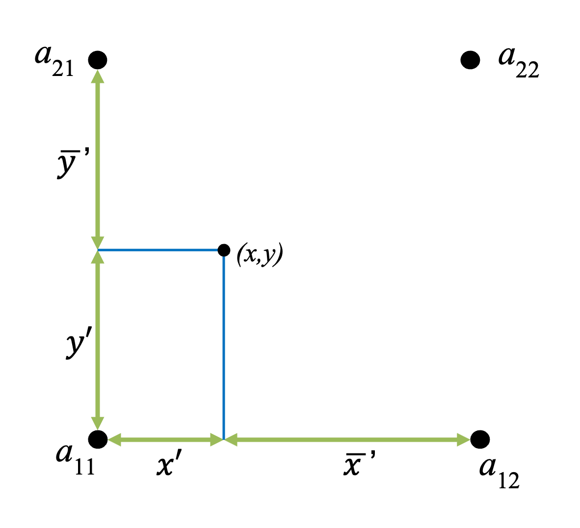
This method requires four valid source points a_ij (1<=i,j<=2) surrounding the point (x,y), to which geogrid or metgrid must interpolate, as illustrated in the figure above. The method works by linearly interpolating to the x-coordinate of the point (x,y) between a₁₁ and a₁₂, and between a₂₁ and a₂₂, and then linearly interpolating to the y-coordinate using these two interpolated values.

sixteen_pt: Sixteen-point Overlapping Parabolic Interpolation¶

This method requires sixteen valid source points surrounding the point (x,y), as illustrated in the figure above. It fits one parabola to the points a_i1, a_i2, and a_i3, and another parabola to the points a_i2, a_i3, and a_i4, for row i, 1<=i<=4; then, an intermediate interpolated value p_i within row i at the x-coordinate of the point is computed by taking an average of the values of the two parabolas evaluated at x, with the average being weighted linearly by the distance of x from a_i2 and a_i3. Finally, the interpolated value at (x,y) is found by performing the same operations as for a row of points, but for the column of interpolated values p_i to the y-coordinate of (x,y).

average_4pt: Simple Four-point Average Interpolation¶

This method requires at least one valid source data point from the four source points surrounding the point (x,y). The interpolated value is the average of all valid values among these four points.

wt_average_4pt: Weighted Four-point Average Interpolation¶

This method can handle missing or masked source data points, and the interpolated value is the weighted average of all valid values, with the weight w_ij for the source point a_ij, 1<=i, j<=2, given by

Here, x_i is the x-coordinate of a_ij and y_j is the y-coordinate of a_ij.

average_16pt: Simple Sixteen-point Average Interpolation¶

This method works identically to the four-point average, but considers the sixteen points surrounding the point (x,y).

wt_average_16pt: Weighten Sixteen-point Average Interpolation¶

This works like the weighted four-point average, but considers the sixteen points surrounding (x,y); the weights in this method are given by

where x_i and y_j are as defined for the weighted four-point method, and 1<=i,j<=4.

nearest_neighbor: Nearest Neighbor Interpolation¶

When used for continuous data sets (those having type=continuous in their index files), this method sets the interpolated value at (x,y) to the value of the nearest source data point, regardless of whether this point is valid, missing, or masked. For categorical data sets (those having type=categorical in their index files), this option considers all source pixels within each WRF grid cell, and finds the fraction of the WRF grid cell that is comprised of each category in the source data.

search: Breadth-first Search Interpolation¶

This option treats the source data array as a 2-d grid graph, where each source data point, whether valid or not, is represented by a vertex. Then, the value assigned to the point (x,y) is found by beginning a breadth-first search at the vertex corresponding to the nearest neighbor of (x,y), and stopping once a vertex representing a valid (i.e., not masked or missing) source data point is found. In effect, this method can be thought of as “nearest valid neighbor”.

average_gcell: Model Grid-cell Average¶

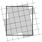
This interpolator may be used when the source data resolution is higher than the model grid resolution. For a model grid cell, T, this method takes an average of the values of all source data points that are nearer to the center of T than to the center of any other grid cell. This is illustrated in the figure above, where the interpolated value for the model grid cell - represented as the large rectangle - is given by the average of the values of all of the shaded source grid cells.

WPS Output¶

Geogrid Output¶

Geogrid output is written in the “WRF I/O API” format. Using the default format setting in namelist.wps (io_format=2), geogrid writes netCDF-formatted output for easy visualization using external software packages, including ncview, NCL, and RIP4.

Below is a listing of the global attributes and fields that are written to the geogrid program’s output files (geo_em.d0x.nc). This is an abridged version of the output when running the ncdump program on a typical geo_em.d01.nc file.

> ncdump -h geo_em.d01.nc

netcdf geo_em.d01 {
dimensions:
        Time = UNLIMITED ; // (1 currently)
        DateStrLen = 19 ;
        west_east = 73 ;
        south_north = 60 ;
        south_north_stag = 61 ;
        west_east_stag = 74 ;
        land_cat = 21 ;
        soil_cat = 16 ;
        month = 12 ;
        num_urb_params = 132 ;
variables:
      char Times(Time, DateStrLen) ;
      float XLAT_M(Time, south_north, west_east) ;
           XLAT_M:units = "degrees latitude" ;
           XLAT_M:description = "Latitude on mass grid" ;
      float XLONG_M(Time, south_north, west_east) ;
           XLONG_M:units = "degrees longitude" ;
           XLONG_M:description = "Longitude on mass grid" ;
      float XLAT_V(Time, south_north_stag, west_east) ;
           XLAT_V:units = "degrees latitude" ;
           XLAT_V:description = "Latitude on V grid" ;
      float XLONG_V(Time, south_north_stag, west_east) ;
           XLONG_V:units = "degrees longitude" ;
           XLONG_V:description = "Longitude on V grid" ;
      float XLAT_U(Time, south_north, west_east_stag) ;
           XLAT_U:units = "degrees latitude" ;
           XLAT_U:description = "Latitude on U grid" ;
      float XLONG_U(Time, south_north, west_east_stag) ;
           XLONG_U:units = "degrees longitude" ;
           XLONG_U:description = "Longitude on U grid" ;
      float CLAT(Time, south_north, west_east) ;
           CLAT:units = "degrees latitude" ;
           CLAT:description = "Computational latitude on mass grid" ;
      float CLONG(Time, south_north, west_east) ;
           CLONG:units = "degrees longitude" ;
           CLONG:description = "Computational longitude on mass grid" ;
      float MAPFAC_M(Time, south_north, west_east) ;
           MAPFAC_M:units = "none" ;
           MAPFAC_M:description = "Mapfactor on mass grid" ;
      float MAPFAC_V(Time, south_north_stag, west_east) ;
           MAPFAC_V:units = "none" ;
           MAPFAC_V:description = "Mapfactor on V grid" ;
      float MAPFAC_U(Time, south_north, west_east_stag) ;
           MAPFAC_U:units = "none" ;
           MAPFAC_U:description = "Mapfactor on U grid" ;
      float MAPFAC_MX(Time, south_north, west_east) ;
           MAPFAC_MX:units = "none" ;
           MAPFAC_MX:description = "Mapfactor (x-dir) on mass grid" ;
      float MAPFAC_VX(Time, south_north_stag, west_east) ;
           MAPFAC_VX:units = "none" ;
           MAPFAC_VX:description = "Mapfactor (x-dir) on V grid" ;
      float MAPFAC_UX(Time, south_north, west_east_stag) ;
           MAPFAC_UX:units = "none" ;
           MAPFAC_UX:description = "Mapfactor (x-dir) on U grid" ;
      float MAPFAC_MY(Time, south_north, west_east) ;
           MAPFAC_MY:units = "none" ;
           MAPFAC_MY:description = "Mapfactor (y-dir) on mass grid" ;
      float MAPFAC_VY(Time, south_north_stag, west_east) ;
           MAPFAC_VY:units = "none" ;
           MAPFAC_VY:description = "Mapfactor (y-dir) on V grid" ;
      float MAPFAC_UY(Time, south_north, west_east_stag) ;
           MAPFAC_UY:units = "none" ;
           MAPFAC_UY:description = "Mapfactor (y-dir) on U grid" ;
      float E(Time, south_north, west_east) ;
           E:units = "-" ;
           E:description = "Coriolis E parameter" ;
      float F(Time, south_north, west_east) ;
           F:units = "-" ;
           F:description = "Coriolis F parameter" ;
      float SINALPHA(Time, south_north, west_east) ;
           SINALPHA:units = "none" ;
           SINALPHA:description = "Sine of rotation angle" ;
      float COSALPHA(Time, south_north, west_east) ;
           COSALPHA:units = "none" ;
           COSALPHA:description = "Cosine of rotation angle" ;
      float LANDMASK(Time, south_north, west_east) ;
           LANDMASK:units = "none" ;
           LANDMASK:description = "Landmask : 1=land, 0=water" ;
      float XLAT_C(Time, south_north_stag, west_east_stag) ;
           XLAT_C:units = "degrees latitude" ;
           XLAT_C:description = "Latitude at grid cell corners" ;
      float XLONG_C(Time, south_north_stag, west_east_stag) ;
           XLONG_C:units = "degrees longitude" ;
           XLONG_C:description = "Longitude at grid cell corners" ;
      float LANDUSEF(Time, land_cat, south_north, west_east) ;
           LANDUSEF:units = "category" ;
           LANDUSEF:description = "Noah-modified 21-category IGBP-MODIS landuse" ;
      float LU_INDEX(Time, south_north, west_east) ;
           LU_INDEX:units = "category" ;
           LU_INDEX:description = "Dominant category" ;
      float HGT_M(Time, south_north, west_east) ;
           HGT_M:units = "meters MSL" ;
           HGT_M:description = "GMTED2010 30-arc-second topography height" ;
      float SOILTEMP(Time, south_north, west_east) ;
           SOILTEMP:units = "Kelvin" ;
           SOILTEMP:description = "Annual mean deep soil temperature" ;
      float SOILCTOP(Time, soil_cat, south_north, west_east) ;
           SOILCTOP:units = "category" ;
           SOILCTOP:description = "16-category top-layer soil type" ;
      float SCT_DOM(Time, south_north, west_east) ;
           SCT_DOM:units = "category" ;
           SCT_DOM:description = "Dominant category" ;
      float SOILCBOT(Time, soil_cat, south_north, west_east) ;
           SOILCBOT:units = "category" ;
           SOILCBOT:description = "16-category top-layer soil type" ;
      float SCB_DOM(Time, south_north, west_east) ;
           SCB_DOM:units = "category" ;
           SCB_DOM:description = "Dominant category" ;
      float ALBEDO12M(Time, month, south_north, west_east) ;
           ALBEDO12M:units = "percent" ;
           ALBEDO12M:description = "Monthly surface albedo" ;
      float GREENFRAC(Time, month, south_north, west_east) ;
           GREENFRAC:units = "fraction" ;
           GREENFRAC:description = "MODIS FPAR" ;
      float LAI12M(Time, month, south_north, west_east) ;
           LAI12M:units = "m^2/m^2" ;
           LAI12M:description = "MODIS LAI" ;
      float SNOALB(Time, south_north, west_east) ;
           SNOALB:units = "percent" ;
           SNOALB:description = "Maximum snow albedo" ;
      float SLOPECAT(Time, south_north, west_east) ;
           SLOPECAT:units = "category" ;
           SLOPECAT:description = "Dominant category" ;
      float CON(Time, south_north, west_east) ;
           CON:units = "" ;
           CON:description = "Subgrid-scale orographic convexity" ;
      float VAR(Time, south_north, west_east) ;
           VAR:units = "" ;
           VAR:description = "Subgrid-scale orographic variance" ;
      float OA1(Time, south_north, west_east) ;
           OA1:units = "" ;
           OA1:description = "Subgrid-scale orographic asymmetry" ;
      float OA2(Time, south_north, west_east) ;
           OA2:units = "" ;
           OA2:description = "Subgrid-scale orographic asymmetry" ;
      float OA3(Time, south_north, west_east) ;
            OA3:units = "" ;
           OA3:description = "Subgrid-scale orographic asymmetry" ;
      float OA4(Time, south_north, west_east) ;
           OA4:units = "" ;
           OA4:description = "Subgrid-scale orographic asymmetry" ;
      float OL1(Time, south_north, west_east) ;
           OL1:units = "" ;
           OL1:description = "Subgrid-scale effective orographic length scale" ;
      float OL2(Time, south_north, west_east) ;
           OL2:units = "" ;
           OL2:description = "Subgrid-scale effective orographic length scale" ;
      float OL3(Time, south_north, west_east) ;
           OL3:units = "" ;
           OL3:description = "Subgrid-scale effective orographic length scale" ;
      float OL4(Time, south_north, west_east) ;
           OL4:units = "" ;
           OL4:description = "Subgrid-scale effective orographic length scale" ;
      float VAR_SSO(Time, south_north, west_east) ;
           VAR_SSO:units = "meters2 MSL" ;
           VAR_SSO:description = "Variance of Subgrid Scale Orography" ;
      float LAKE_DEPTH(Time, south_north, west_east) ;
           LAKE_DEPTH:units = "meters MSL" ;
           LAKE_DEPTH:description = "Topography height" ;
      float URB_PARAM(Time, num_urb_params, south_north, west_east) ;
           URB_PARAM:units = "dimensionless" ;
           URB_PARAM:description = "Urban_Parameters" ;

// global attributes:
           :TITLE = "OUTPUT FROM GEOGRID V4.0" ;
           :SIMULATION_START_DATE = "0000-00-00_00:00:00" ;
           :WEST-EAST_GRID_DIMENSION = 74 ;
           :SOUTH-NORTH_GRID_DIMENSION = 61 ;
           :BOTTOM-TOP_GRID_DIMENSION = 0 ;
           :WEST-EAST_PATCH_START_UNSTAG = 1 ;
           :WEST-EAST_PATCH_END_UNSTAG = 73 ;
           :WEST-EAST_PATCH_START_STAG = 1 ;
           :WEST-EAST_PATCH_END_STAG = 74 ;
           :SOUTH-NORTH_PATCH_START_UNSTAG = 1 ;
           :SOUTH-NORTH_PATCH_END_UNSTAG = 60 ;
           :SOUTH-NORTH_PATCH_START_STAG = 1 ;
           :SOUTH-NORTH_PATCH_END_STAG = 61 ;
           :GRIDTYPE = "C" ;
           :DX = 30000.f ;
           :DY = 30000.f ;
           :DYN_OPT = 2 ;
           :CEN_LAT = 34.83001f ;
           :CEN_LON = -81.03f ;
           :TRUELAT1 = 30.f ;
           :TRUELAT2 = 60.f ;
           :MOAD_CEN_LAT = 34.83001f ;
           :STAND_LON = -98.f ;
           :POLE_LAT = 90.f ;
           :POLE_LON = 0.f ;
           :corner_lats = 28.17127f, 44.36657f, 39.63231f, 24.61906f, 28.17842f, 44.37617f, \
           39.57812f, 24.57806f, 28.03771f, 44.50592f, 39.76032f, 24.49431f, 28.04485f, \
           44.51553f, 39.70599f, 24.45341f ;
           :corner_lons = -93.64893f, -92.39661f, -66.00165f, -72.64047f, -93.80048f, \
           -92.59155f, -65.83557f, -72.5033f, -93.65717f, -92.3829f, -65.9313f, \
           -72.68539f, -93.80841f, -92.57831f, -65.76495f, -72.54843f ;
           :MAP_PROJ = 1 ;
           :MMINLU = "MODIFIED_IGBP_MODIS_NOAH" ;
           :NUM_LAND_CAT = 21 ;
           :ISWATER = 17 ;
           :ISLAKE = 21 ;
           :ISICE = 15 ;
           :ISURBAN = 13 ;
           :ISOILWATER = 14 ;
           :grid_id = 1 ;
           :parent_id = 1 ;
           :i_parent_start = 1 ;
           :j_parent_start = 1 ;
           :i_parent_end = 74 ;
           :j_parent_end = 61 ;
           :parent_grid_ratio = 1 ;
           :FLAG_MF_XY = 1 ;
           :FLAG_LAI12M = 1 ;
           :FLAG_LAKE_DEPTH = 1 ;
}

Global attributes corner_lats and corner_lons contain the lat-lon location of the domain’s corners with respect to different grid staggerings (mass, u, v, and unstaggered). The locations referred to by each element of the corner_lats and corner_lons arrays are summarized in the table and figure below.

../../_images/wps_corner_lats_lons_table.png

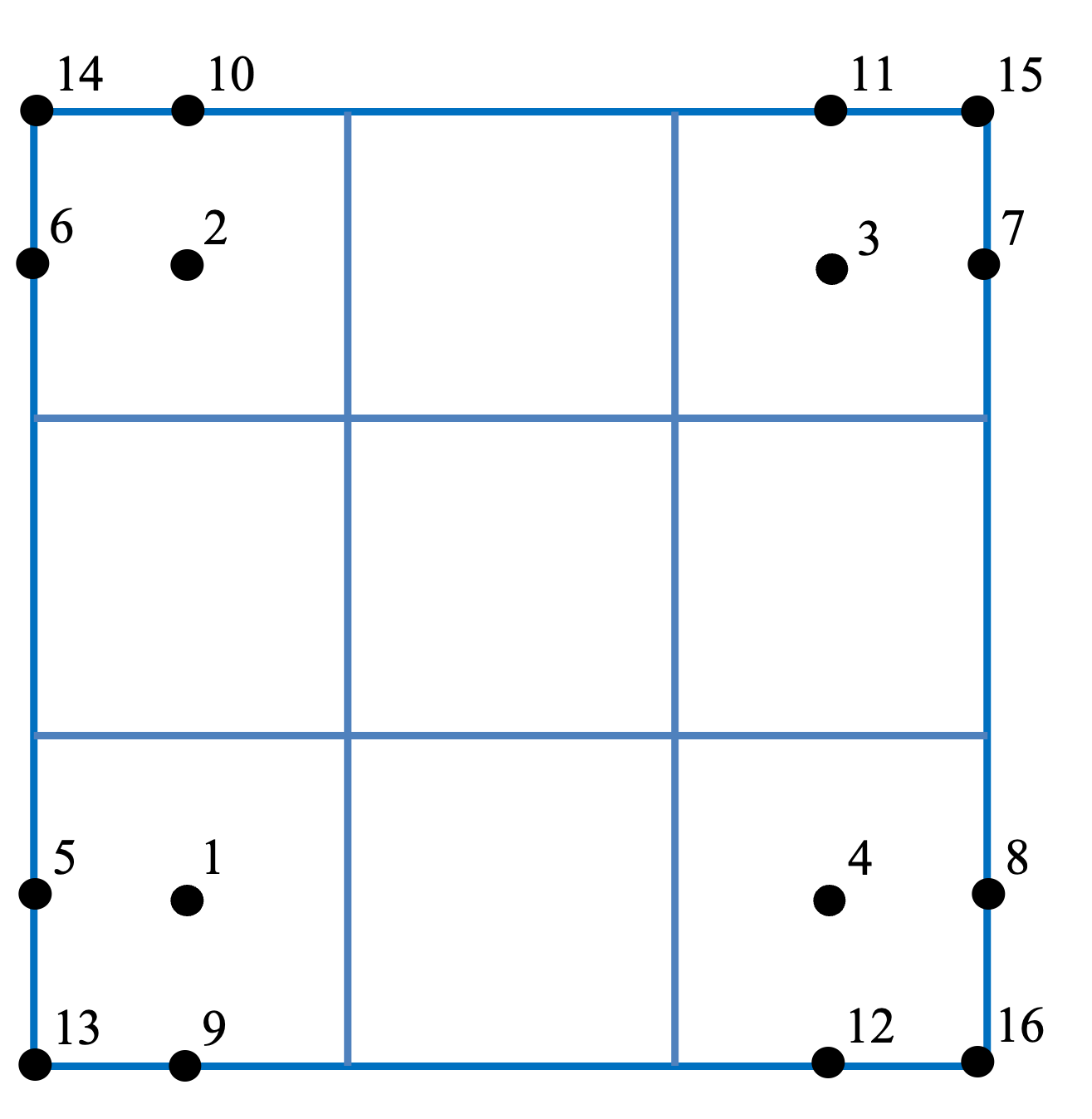
Metgrid Output¶

Output from the metgrid program is in the form of met_em.d0x.YYYY-MM-DD_hh:mm:ss.xx, using the following naming convention:

met_em: Signifies data output from the WPS metgrid.exe program and input into the real.exe program
d01: Identifies to which domain the file refers (nests follow the convection “d02,” “d03,” etc.)
YYYY-MM-DD_hh:mm:ss: The UTC validation date/time, specified as YEAR-MONTH-DAY_hour:minute:second, where each WPS output file has only a single time-slice of processed data
.nc: The file extension indicating the metgrid output format. .nc indicates this is a netCDF file, which is the default format.

In addition to the fields contained in a geogrid output file (e.g., geo_em.d01.nc), the following fields and global attributes will also be present in a typical output file from the metgrid program.

Note

The below file content was produced using the default METGRID.TBL file and meteorological data from NCEP’s GFS model.

> ncdump met_em.d01.2016-04-07_00:00:00.nc

netcdf met_em.d01.2016-04-07_00\:00\:00 {
dimensions:
Time = UNLIMITED ; // (1 currently)
      DateStrLen = 19 ;
      west_east = 73 ;
      south_north = 60 ;
      num_metgrid_levels = 27 ;
      num_st_layers = 4 ;
      num_sm_layers = 4 ;
      south_north_stag = 61 ;
      west_east_stag = 74 ;
      z-dimension0132 = 132 ;
      z-dimension0012 = 12 ;
      z-dimension0016 = 16 ;
      z-dimension0021 = 21 ;
variables:
      char Times(Time, DateStrLen) ;
      float PRES(Time, num_metgrid_levels, south_north, west_east) ;
           PRES:units = "" ;
           PRES:description = "" ;
      float SOIL_LAYERS(Time, num_st_layers, south_north, west_east) ;
           SOIL_LAYERS:units = "" ;
           SOIL_LAYERS:description = "" ;
      float SM(Time, num_sm_layers, south_north, west_east) ;
           SM:units = "" ;
           SM:description = "" ;
      float ST(Time, num_st_layers, south_north, west_east) ;
           ST:units = "" ;
           ST:description = "" ;
      float GHT(Time, num_metgrid_levels, south_north, west_east) ;
           GHT:units = "m" ;
           GHT:description = "Height" ;
      float HGTTROP(Time, south_north, west_east) ;
           HGTTROP:units = "m" ;
           HGTTROP:description = "Height of tropopause" ;
      float TTROP(Time, south_north, west_east) ;
           TTROP:units = "K" ;
           TTROP:description = "Temperature at tropopause" ;
      float PTROPNN(Time, south_north, west_east) ;
           PTROPNN:units = "Pa" ;
           PTROPNN:description = "PTROP, used for nearest neighbor interp" ;
      float PTROP(Time, south_north, west_east) ;
           PTROP:units = "Pa" ;
           PTROP:description = "Pressure of tropopause" ;
      float VTROP(Time, south_north_stag, west_east) ;
           VTROP:units = "m s-1" ;
           VTROP:description = "V at tropopause" ;
      float UTROP(Time, south_north, west_east_stag) ;
           UTROP:units = "m s-1" ;
           UTROP:description = "U at tropopause" ;
      float HGTMAXW(Time, south_north, west_east) ;
           HGTMAXW:units = "m" ;
           HGTMAXW:description = "Height of max wind level" ;
      float TMAXW(Time, south_north, west_east) ;
           TMAXW:units = "K" ;
           TMAXW:description = "Temperature at max wind level" ;
      float PMAXWNN(Time, south_north, west_east) ;
           PMAXWNN:units = "Pa" ;
           PMAXWNN:description = "PMAXW, used for nearest neighbor interp" ;
      float PMAXW(Time, south_north, west_east) ;
           PMAXW:units = "Pa" ;
           PMAXW:description = "Pressure of max wind level" ;
      float VMAXW(Time, south_north_stag, west_east) ;
           VMAXW:units = "m s-1" ;
           VMAXW:description = "V at max wind" ;
      float UMAXW(Time, south_north, west_east_stag) ;
           UMAXW:units = "m s-1" ;
           UMAXW:description = "U at max wind" ;
      float SNOWH(Time, south_north, west_east) ;
           SNOWH:units = "m" ;
           SNOWH:description = "Physical Snow Depth" ;
      float SNOW(Time, south_north, west_east) ;
           SNOW:units = "kg m-2" ;
           SNOW:description = "Water equivalent snow depth" ;
      float SKINTEMP(Time, south_north, west_east) ;
           SKINTEMP:units = "K" ;
           SKINTEMP:description = "Skin temperature" ;
      float SOILHGT(Time, south_north, west_east) ;
           SOILHGT:units = "m" ;
           SOILHGT:description = "Terrain field of source analysis" ;
      float LANDSEA(Time, south_north, west_east) ;
           LANDSEA:units = "proprtn" ;
           LANDSEA:description = "Land/Sea flag (1=land, 0 or 2=sea)" ;
      float SEAICE(Time, south_north, west_east) ;
           SEAICE:units = "proprtn" ;
           SEAICE:description = "Ice flag" ;
      float ST100200(Time, south_north, west_east) ;
           ST100200:units = "K" ;
           ST100200:description = "T 100-200 cm below ground layer (Bottom)" ;
      float ST040100(Time, south_north, west_east) ;
           ST040100:units = "K" ;
           ST040100:description = "T 40-100 cm below ground layer (Upper)" ;
      float ST010040(Time, south_north, west_east) ;
           ST010040:units = "K" ;
           ST010040:description = "T 10-40 cm below ground layer (Upper)" ;
      float ST000010(Time, south_north, west_east) ;
           ST000010:units = "K" ;
           ST000010:description = "T 0-10 cm below ground layer (Upper)" ;
      float SM100200(Time, south_north, west_east) ;
           SM100200:units = "fraction" ;
           SM100200:description = "Soil Moist 100-200 cm below gr layer" ;
      float SM040100(Time, south_north, west_east) ;
           SM040100:units = "fraction" ;
           SM040100:description = "Soil Moist 40-100 cm below grn layer" ;
      float SM010040(Time, south_north, west_east) ;
           SM010040:units = "fraction" ;
           SM010040:description = "Soil Moist 10-40 cm below grn layer" ;
      float SM000010(Time, south_north, west_east) ;
           SM000010:units = "fraction" ;
           SM000010:description = "Soil Moist 0-10 cm below grn layer (Up)" ;
      float PSFC(Time, south_north, west_east) ;
           PSFC:units = "Pa" ;
           PSFC:description = "Surface Pressure" ;
      float RH(Time, num_metgrid_levels, south_north, west_east) ;
           RH:units = "%" ;
           RH:description = "Relative Humidity" ;
      float VV(Time, num_metgrid_levels, south_north_stag, west_east) ;
           VV:units = "m s-1" ;
           VV:description = "V" ;
      float UU(Time, num_metgrid_levels, south_north, west_east_stag) ;
           UU:units = "m s-1" ;
           UU:description = "U" ;
      float TT(Time, num_metgrid_levels, south_north, west_east) ;
           TT:units = "K" ;
           TT:description = "Temperature" ;
      float PMSL(Time, south_north, west_east) ;
           PMSL:units = "Pa" ;
           PMSL:description = "Sea-level Pressure" ;

// global attributes:
           :TITLE = "OUTPUT FROM METGRID V4.0" ;
           :SIMULATION_START_DATE = "2016-04-07_00:00:00" ;
           :WEST-EAST_GRID_DIMENSION = 74 ;
           :SOUTH-NORTH_GRID_DIMENSION = 61 ;
           :BOTTOM-TOP_GRID_DIMENSION = 27 ;
           :WEST-EAST_PATCH_START_UNSTAG = 1 ;
           :WEST-EAST_PATCH_END_UNSTAG = 73 ;
           :WEST-EAST_PATCH_START_STAG = 1 ;
           :WEST-EAST_PATCH_END_STAG = 74 ;
           :SOUTH-NORTH_PATCH_START_UNSTAG = 1 ;
           :SOUTH-NORTH_PATCH_END_UNSTAG = 60 ;
           :SOUTH-NORTH_PATCH_START_STAG = 1 ;
           :SOUTH-NORTH_PATCH_END_STAG = 61 ;
           :GRIDTYPE = "C" ;
           :DX = 30000.f ;
           :DY = 30000.f ;
           :DYN_OPT = 2 ;
           :CEN_LAT = 34.83001f ;
           :CEN_LON = -81.03f ;
           :TRUELAT1 = 30.f ;
           :TRUELAT2 = 60.f ;
           :MOAD_CEN_LAT = 34.83001f ;
           :STAND_LON = -98.f ;
           :POLE_LAT = 90.f ;
           :POLE_LON = 0.f ;
           :corner_lats = 28.17127f, 44.36657f, 39.63231f, 24.61906f, 28.17842f, \
           44.37617f, 39.57812f, 24.57806f, 28.03771f, 44.50592f, 39.76032f, 24.49431f, \
           28.04485f, 44.51553f, 39.70599f, 24.45341f ;
           :corner_lons = -93.64893f, -92.39661f, -66.00165f, -72.64047f, -93.80048f, \
           -92.59155f, -65.83557f, -72.5033f, -93.65717f, -92.3829f, -65.9313f, \
           -72.68539f, -93.80841f, -92.57831f, -65.76495f, -72.54843f ;
           :MAP_PROJ = 1 ;
           :MMINLU = "MODIFIED_IGBP_MODIS_NOAH" ;
           :NUM_LAND_CAT = 21 ;
           :ISWATER = 17 ;
           :ISLAKE = 21 ;
           :ISICE = 15 ;
           :ISURBAN = 13 ;
           :ISOILWATER = 14 ;
           :grid_id = 1 ;
           :parent_id = 1 ;
           :i_parent_start = 1 ;
           :j_parent_start = 1 ;
           :i_parent_end = 74 ;
           :j_parent_end = 61 ;
           :parent_grid_ratio = 1 ;
           :NUM_METGRID_SOIL_LEVELS = 4 ;
           :FLAG_METGRID = 1 ;
           :FLAG_EXCLUDED_MIDDLE = 0 ;
           :FLAG_SOIL_LAYERS = 1 ;
           :FLAG_SNOW = 1 ;
           :FLAG_PSFC = 1 ;
           :FLAG_SM000010 = 1 ;
           :FLAG_SM010040 = 1 ;
           :FLAG_SM040100 = 1 ;
           :FLAG_SM100200 = 1 ;
           :FLAG_ST000010 = 1 ;
           :FLAG_ST010040 = 1 ;
           :FLAG_ST040100 = 1 ;
           :FLAG_ST100200 = 1 ;
           :FLAG_SLP = 1 ;
           :FLAG_SNOWH = 1 ;
           :FLAG_SOILHGT = 1 ;
           :FLAG_UTROP = 1 ;
           :FLAG_VTROP = 1 ;
           :FLAG_TTROP = 1 ;
           :FLAG_PTROP = 1 ;
           :FLAG_PTROPNN = 1 ;
           :FLAG_HGTTROP = 1 ;
           :FLAG_UMAXW = 1 ;
           :FLAG_VMAXW = 1 ;
           :FLAG_TMAXW = 1 ;
           :FLAG_PMAXW = 1 ;
           :FLAG_PMAXWNN = 1 ;
           :FLAG_HGTMAXW = 1 ;
           :FLAG_MF_XY = 1 ;
           :FLAG_LAI12M = 1 ;
           :FLAG_LAKE_DEPTH = 1 ;
}

Checking WPS Output¶

It can be helpful to examine WPS output. For example,

Viewing the interpolated static geographical data and latitude/longitude fields when determining the location of nests
When importing a new static or meteorological data source into WPS, it can be beneficial to check the resulting interpolated fields in order to make adjustments to the interpolation methods used by geogrid or metgrid

Checking Geogrid & Metgrid Output¶

A variety of visualization tools capable of reading netCDF files may be utilized if geogrid and metgrid output are in netCDF format. To ensure output files are in netCDF format, set the following namelist options to 2 (which is the default setting).

&share
  io_form_geogrid = 2,
/

&metgrid
  io_form_metgrid = 2,
/

The following programs may be of interest.

ncdump
A compact utility distributed with netCDF libraries that lists variables and attributes in netCDF files. This can be useful for checking domain parameters (e.g., west-east dimension, south-north dimension, or domain center point) in geogrid output, or for listing the fields in a file.
ncview
Provides an interactive way to view fields in netCDF files, and/or for producing plots suitable for use in publications
Read/Interpolate/Plot (RIP) (Read/Interpolate/Plot)
Plots horizontal contours, map backgrounds, and overlaying multiple fields within the same plot

Checking Ungrib Output¶

Ungrib output is written in a simple binary format (either ‘WPS’, ‘SI’, or ‘MM5’), so software for viewing netCDF files cannot be used for ungrib output. However, the following tools are provided with WPS source code (found in the util directory):

plotfmt
An NSF NCAR Graphics-based utility that produces contour plots of fields available in intermediate-formatted files. If the NCAR Graphics libraries are properly installed, this program is automatically compiled when WPS is built.
rd_intermediate.exe
Prints information about fields contained in ungrib output

Using MPAS Output for WRF Input¶

Output from MPAS may be used to provide initial and lateral boundary conditions for WRF. The metgrid.exe program is capable of reading native, unstructured mesh netCDF output from the Model for Prediction Across Scales (MPAS). Metgrid can horizontally interpolate the MPAS fields directly to any domain defined by the geogrid program, to produce output files usable by the WRF real.exe program in the same way as metgrid output interpolated from intermediate files.

When running an MPAS simulation, an output stream must be set to contain the minimum set of fields necessary to initialize a WRF simulation. The following output stream should be sufficient with MPAS v5 and later code.

<stream name="wrf_ic_bc"
        type="output"
        filename_template="MPAS.$Y-$M-$D_$h.nc"
        output_interval="3:00:00" >

 <var name="xtime"/>
 <var_array name="scalars"/>
 <var name="pressure"/>
 <var name="zgrid"/>
 <var name="theta"/>
 <var name="uReconstructZonal"/>
 <var name="uReconstructMeridional"/>
 <var name="u10"/>
 <var name="v10"/>
 <var name="q2"/>
 <var name="t2m"/>
 <var name="skintemp"/>
 <var name="surface_pressure"/>
 <var name="mslp"/>
 <var name="tslb"/>
 <var name="smois"/>

</stream>

After running MPAS with a suitable output stream defined, netCDF files are produced that contain fields on the native MPAS mesh. Because these files do not include fields describing the locations, geometry, and connectivity of the MPAS grid cells, this information must be provided to the metgrid program with a ‘static’ file from the MPAS simulation. The MPAS netCDF files (prefixed with mpas) must be specified in the &metgrid namelist record, for both the constants_name and fg_name variables, e.g.,

&metgrid
  constants_name = 'mpas:static.nc'
  fg_name = 'mpas:MPAS'
/

Given the above example, metgrid reads the MPAS static.nc file to gather mesh information and compute remapping weights from the MPAS mesh to the WRF domain, defined by the geogrid program, then processes all time periods from the MPAS files with prefix MPAS (and suffix YYYY-MM-DD_HH.nc). Afterward the real.exe program is run as usual.

Note

The use of native MPAS output with metgrid.exe has not been thoroughly tested for parallel (i.e., dmpar) builds of the WPS; it is therefore recommended to run metgrid.exe serially when processing MPAS data sets.

Combining Intermediate and MPAS Data¶

Intermediate file data (created by the ungrib program) can be combined with MPAS data by the metgrid program. This may be useful, e.g., to use SST, sea ice, or land-surface fields from another source. The following example combines MPAS data with ERA-Interim intermediate files with soil data (with prefix ERAI_SOIL).

&metgrid
  constants_name = 'mpas:static.nc'
  fg_name = 'mpas:MPAS', 'ERAI_SOIL'
/

Omitting the MPAS zgrid Field¶

Because the MPAS zgrid field does not change in time, it can be omitted from the MPAS periodic output stream. To do so, the zgrid field is placed in its own netCDF file that defines the Time dimension as a netCDF unlimited dimension. Then, this file (say, zgrid.nc) can be supplied to the metgrid program using the constants_name namelist variable, e.g.,

&metgrid
  constants_name = 'mpas:static.nc', 'mpas:zgrid.nc'
  fg_name = 'mpas:MPAS'
/

Placing zgrid in its own file can save considerable space when long MPAS simulations are run, or when the output stream to be used as WRF initial and boundary conditions is written out at high temporal frequency. The python script below serves as an example for extracting the zgrid field to its own netCDF file.

from netCDF4 import Dataset

fin = Dataset('init.nc')
fout = Dataset('zgrid.nc','w',format='NETCDF3_64BIT')

nCells = fin.dimensions['nCells'].size
nVertLevelsP1 = fin.dimensions['nVertLevelsP1'].size

fout.createDimension(dimname='Time',size=None)
fout.createDimension(dimname='nCells',size=nCells)
fout.createDimension(dimname='nVertLevelsP1',size=nVertLevelsP1)
fout.createVariable(varname='zgrid',datatype='f',dimensions=('nCells', 'nVertLevelsP1'))
fout.variables['zgrid'][:] = fin.variables['zgrid'][:]
fout.close()
fin.close()

Using MPAS Output with Large Meshes¶

In cases of large MPAS meshes, it may be necessary to increase the value of two constants in the metgrid code that are used to statically allocate several data structures used in computation of remapping weights from the MPAS mesh to the WRF domain. These two constants, shown below, are located in the WPS/src/metgrid/remapper.F file.

! should be at least (earth circumference / minimum grid distance)
integer, parameter :: max_queue_length    = 2700

! should be at least (nCells/32)
integer, parameter :: max_dictionary_size = 82000

After changing the value of these constants, metgrid must be recompiled.