OBSGRID¶

The OBSGRID utility is an objective analysis tool, used specifically with WRF, that incorporates observations to improve meteorological analysis.

Traditionally, these observations have been ‘direct’ observations of temperature, humidity, and wind from surface and radiosonde reports. As remote sensing techniques are advancing, more ‘indirect’ observations are available. Effective use of these indirect observations for objective analysis is not a trivial task. Methods commonly employed for indirect observations include three-dimensional or four-dimensional variational techniques (3DVAR and 4DVAR, respectively), which can be used for direct observations as well.

OBSGRID Program Flow¶

../../_images/utilities_obsgrid_flow.png

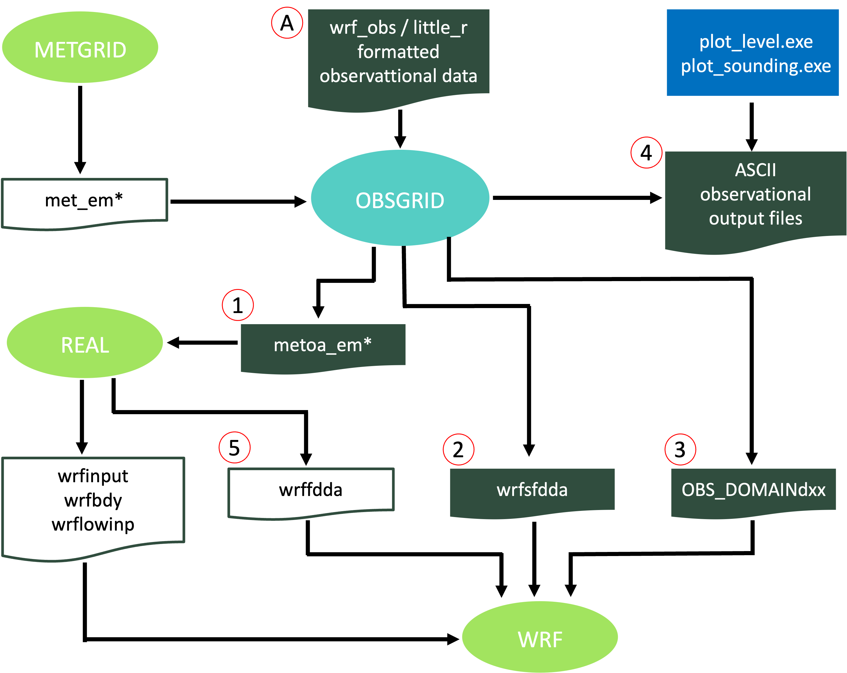
The OBSGRID utility is run after metgrid.exe. It uses the metgrid output (met_em files), as well as additional observations as input. See Format of Observations to read more about the observational file format.

Output from the objective analysis programs can be used to provide:

metoa_em.d0x : Fields for initial and boundary conditions . These files have identical formatting as the met_em* files from metgrid.exe. However, metoa_em files also incorporate observational information.
wrfsdffa_d0x : Surface fields for surface-analysis-nudging FDDA . When using this file as input to WRF, it is recommended to also use the 3-D fdda file (wrffdda , which is an optional output file created when running real.exe) as input to WRF.
OBS_DOMAINd0x : Data for observational nudging . Note - since OBSGRID version 3.1.1, this file can be read directly by the observational nudging code and no longer needs to pass through an additional perl script.
ASCII and netCDF output (.tttt or .nc files) . These files contain observation information and the assigned quality control flags. These files can be plotted with the provided plotting utilities.

Source of Observations¶

OBSGRID reads observations that have been formatted as ASCII text files (wrf_obs / little_r format) by the user. This allows users to adapt their own data to be used as input to the OBSGRID program.

Programs are available to convert NMC ON29 and NCEP BUFR formatted files into the ‘wrf_obs / little_r’ format. If incorporating other other observations into OBSGRID, users are responsible for converting the data into this format.

Note

See the OBSGRID/util directory for a user-contributed (i.e., unsupported) program that converts observation files from GTS to ‘wrf_obs / little_r’ format.

NCEP operational global surface and upper-air observation subsets, as archived by NSF NCAR’s Research Data Archive (RDA).

Upper-air data in NMC ON29 format (from early 1970s to early 2000)
Surface data in NMC ON29 format (from early 1970s to early 2000)
Upper-air data in NCEP BUFR format (from 1999 to present)
Surface data in NCEP BUFR format (from 1999 to present)

ds351.0 and ds461.0 data is also available in little_r format. From outside NSF NCAR, these data can be downloaded from the web, and for NSF NCAR supercomputer users, it is available on the glade file system. These data are sorted into 6-hourly windows, creating files that are typically too large for use in OBSGRID. To reorder the files into 3-hourly windows:

Obtain the little_r 6-hourly data:
- Non-NSF NCAR HPC users : Data can be downloaded from the above web sites. Combine (by using the Unix cat command) all surface and upper-air data into a single file called rda_obs.
- NSF NCAR HPC users : Use the script util/get_rda_data.csh, to obtain data and create the file rda_obs. This script must be edited to specify the simulation date range.
Compile the Fortran program util/get_rda_data.f. Place the rda_obs file in the top OBSGRID/ directory. Run util/get_rda_data.exe, which uses the date range from namelist.oa to create 3-hourly OBS:<date> files, which are ready to use in OBSGRID.

As an alternative, observations may be downloaded from Meteorological Assimilation Data Ingest System (MADIS) and then converted to little_r format using the MADIS2LITTLER tool provided by NSF NCAR.

Note

To ensure single-level above-surface observations are handled properly by OBSGRID, MADIS2LITTLER must be modified to mark such observations as soundings (in module_output.F, and in subroutine write_littler_onelvl, set is_sound=.true.).

Objective Analysis Techniques in OBSGRID¶

Cressman Scheme¶

Three of the four objective analysis techniques used in OBSGRID are based on the Cressman scheme, in which several successive scans nudge a first-guess field toward the neighboring observed values. The standard Cressman scheme assigns to each observation a circular radius of influence, \(R\). The first-guess field at each grid point, \(P\), is adjusted by taking into account all the observations that influence \(P\). The differences between the first-guess field and the observations are calculated, and a distance-weighted average of these difference values is added to the value of the first-guess at \(P\). Once all grid points have been adjusted, the adjusted field is used as the first guess for another adjustment cycle. Each subsequent pass uses a smaller radius of influence.

../../_images/utilities_obsgrid_cressman.png

Ellipse Scheme¶

In analyses of wind and relative humidity (fields strongly deformed by the wind) at pressure levels, the circles from the standard Cressman scheme are elongated into ellipses, oriented along the flow. The stronger the wind, the greater the eccentricity of the ellipses. This scheme reduces to the circular Cressman scheme under low-wind conditions.

../../_images/utilities_obsgrid_ellipse.png

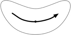
Banana Scheme¶

In analyses of wind and relative humidity at pressure levels, the circles from the standard Cressman scheme are elongated in the direction of the flow, and curved along the streamlines. The result is a banana shape. This scheme reduces to the Ellipse scheme under straight-flow conditions, and the standard Cressman scheme under low-wind conditions.

../../_images/utilities_obsgrid_banana.jpg

Multiquadric Scheme¶

The Multiquadric scheme uses hyperboloid radial basis functions to perform objective analysis. Details of this technique can be found in Nuss and Titley, 1994.

Note

Use this scheme with caution, as it can produce some odd results in areas where only a few observations are available.

Quality Control for Observations¶

OBSGRID screens for bad observations. Many of these quality control checks are optional in OBSGRID.

Quality Control on Individual Reports¶

Gross Error Checks (same values, pressure decreases with height, etc.)
Removes spikes from temperature and wind profiles
Adjusts temperature profiles to remove superadiabatic layers
No comparisons to other reports or to the first-guess field

The ERRMAX Test¶

The ERRMAX quality control check is optional, but is highly recommended.

Limited user control over data removal - the user may set thresholds, which vary the tolerance of the error check
Observations are compared to the first-guess field
If the difference value (\(obs - first\_guess\)) exceeds a certain threshold, the observation is discarded
Threshold varies depending on the field, level, and time of day
Works well with a good first-guess field

The Buddy Test¶

The Buddy Test is optional, but is highly recommended.

Limited user control over data removal - the user may set weighting factors, which vary the tolerance of the error check
Observations are compared to both the first guess and neighboring observations
If the difference value of an observation (\(obs - first\_guess\)) varies significantly from the distance-weighted average of the difference values of neighboring observations, the observation is discarded
Works well in regions with good data density

Additional Observations¶

At times, it may be useful to input additional observations, or to modify existing and erroneous observations.

In OBSGRID, additional observations are provided to the program in the same wrf_obs / little_r format as standard observations. Additional observations must be in the same file as all other observations. Modifying existing/erroneous observations is fairly simple, given that the observation input format is ASCII text. Identifying an observation report as “bogus” simply means that it is assumed to be good data, but no quality control is performed for that report.

Surface FDDA Option¶

The surface FDDA option creates additional surface-only analysis files, usually with a smaller time interval between analyses (i.e., more frequently) than the full upper-air analyses. Surface analysis files can then be used in WRF along with the surface analysis nudging option.

The LAGTEM option controls how the first-guess field is created for surface analysis files. Typically, the surface and upper-air first-guess (analysis times) data are available at twelve-hour or six-hour intervals, while the surface analysis interval may be 3 hours (10800 seconds). So at analysis times, the available surface first-guess is used. If LAGTEM is set to .false., the surface first-guess at other times is temporally interpolated from the first-guess at the analysis times. If LAGTEM=.true., the surface first guess at other times is the objective analysis from the previous time.

Objective Analysis on Model Nests¶

OBSGRID has the capability to perform objective analysis on a nest. This is done manually with a separate OBSGRID process, performed on met_em_d0* files for the particular nest.

Doing objective analysis on a nest can be useful if observations are available with a horizontal resolution somewhat greater than the resolution of the coarse domain. There may also be circumstances in which the representation of terrain on a nest allows for better use of surface observations (i.e., the model terrain better matches the real terrain elevation of the observation).

Note

More often, objective analysis on a nest introduces inconsistency in initial conditions between the coarse domain and the nest. Observations that fall just outside a nest are used in the coarse domain analysis, but are discarded in the nest analysis. Differing observations at a nest boundary can produce very different analyses.

How to Run OBSGRID¶

Obtain OBSGRID Source Code¶

Obtain OBSGRID source code from NSF NCAR’S OBSGRID GitHub Repository or from the WRF Post-processing and Utility Software Download Page. If downloading the file from the webpage, unpack the file (gunzip OBSGRID.TAR.gz and then tar -xf OBSGRID.TAR), which creates a new OBSGRID/ directory.

Generate the OBSGRID Executable¶

NetCDF is the only library required to build OBSGRID. NetCDF source code, precompiled binaries, and documentation are available from Unidata.

If planning to compile the optional utilities plot_level.exe and plot_sounding.exe, NCAR Graphics must also be installed. These utilities are not required to run OBSGRID, but can be useful for displaying observations. Since OBSGRID version 3.7.0, NCL scripts are available and therefore these two utilities are no longer needed to plot the data.

Use the following steps to build OBSGRID:

Configure the code.
```
./configure
```
Choose one of the configure options, then compile.
```
./compile
```

If successful, obsgrid.exe is created in the top-level OBSGRID/ directory. Executables plot_level.exe and plot_sounding.exe are created if NCAR Graphics is installed.

Prepare the Observation Files¶

It is the user’s responsibility to preparing the observational files. Some data are available from NSF NCAR’s Research Data Archive. Data from the early 1970s are in ON29 format, while data from 1999 to present are in NCEP BUFR format. For additional information and/or help using these datasets, see the Source of Observations.

Note

gts_cleaner.f is an unsupported program for reformatting observations from the GTS stream. It is located in in OBSGRID/util. The code expects to find one observational input file per analysis time. Each file should contain both surface and upper-air data (if available).

Edit the OBSGRID Namelist¶

The OBSGRID namelist, namelist.oa, resides in the top-level OBSGRID/ directory. Settings for the start/end dates and file names must be modified for the specific case.

Note

Pay attention to file name settings. Mistakes in observation file names can be overlooked and OBSGRID may process the wrong files. If there are no data in the (wrongly-specified) file for a particular time, OBSGRID provides an analysis of no observations.

Run OBSGRID¶

To run OBSGRID, issue the command:

./obsgrid.exe >& obsgrid.out

The obsgrid.out file provides information and runtime errors. This file name is the user’s choice.

Check Output¶

Examine obsgrid.out for error or warning messages.
OBSGRID should have created metoa_em files. Additional output files containing information about observations found, used, and discarded are created, as well.
Check obsgrid.out for the number of observations found in the objective analysis, and the number of observations used at various levels. This can provide information regarding problems specifying observation files or time intervals.

Plot Utility Programs are also available.

Output Files¶

OBSGRID generates ASCII/netCDF files that detail the actions taken on observations through a time cycle of the program. Files are also created to support plotting the observations for each variable (at each level, at each time). The ASCII/netCDF files are intended for consumption by developers for diagnostic purposes. The primary output of the OBSGRID program is the gridded, pressure-level data that is passed to the real.exe program (files metoa_em).

In each of the files listed below, the text .dn.YYYY-MM-DD_HH:mm:ss.tttt allows a separate output file for each time period processed by OBSGRID. The final four letters tttt indicate the decimal time to ten thousandths of a second. These files are dependent on the domain being processed.

metoa_em¶

metoa_em

The final analysis at surface and pressure levels.

Generating these files is the primary goal of running OBSGRID. They can be used alternatively to the WPS met_em* files to generate WRF initial and boundary conditions. To use these files, when running real.exe, either:

Rename or link the metoa_em* files back to met_em*, which allows real.exe to read the files.
Use the auxinput1_inname option in WRF’s namelist.input file to overwrite the default filename real.exe uses. To do this, prior to running real.exe, add the following to the &time_control namelist record (use the exact syntax as below - do not substitute <domain> and <date> for actual numbers):
```
auxinput1_inname = "metoa_em.d<domain>.<date>"
```

wrfsfdda_dxx¶

wrfsfdda_dxx

A file containing surface analyses at “INTF4D” intervals, analyses of T, TH, U, V, RH, QV, PSFC, PMSL, and a number of observations within 250 km of each grid point

Due to WRF model input requirements, data at the current time (_OLD) and for the next time (_NEW) are supplied at each time interval. Therefore it is important to specify the same surface nudging interval in the &fdda record in WRF’s namelist.input as the interval used in OBSGRID to create the wrfsfdda_d* file.

Data may also need to be available for OBSGRID to create a surface analysis beyond the final WRF surface analysis nudging time. Although the _OLD filed is nudged throughout the rampdown, when the rampdown length is a positive value, WRF requires a _NEW field at the beginning of the rampdown period.

OBS_DOMAINdxx¶

OBS_DOMAINdxx

Files containing a list of all available observations to the OBSGRID program. These files can be used for observational nudging in WRF.

d in the file name represents “domain number”, while xx is the sequential number for the domain (e.g., d01 = domain 1).

ASCII and NetCDF Files (.tttt & .nc)¶

qc_obs_raw.dn.YYYY-MM-DD_HH:mm:ss.tttt(.nc)

A file containing a list of all of the observations available to the OBSGRID program

qc_obs_used.dn.YYYY-MM-DD-HH:mm:ss.tttt(.nc)

A file containing a list of all of the observations used by the OBSGRID program (the same data saved to the OBS_DOMAINdxx files)

qc_obs_used_earth_relative.dn.YYYY-MM-DD-HH:mm:ss.tttt(.nc)

A file containing a list of all the observations used by OBSGRID (the same data saved to the OBS_DOMAINdxx files), but the winds are in an earth-relative framework rather than a model-relative framework. The non-netCDF version of these files can be used as input to the Model Evaluation Tools (MET) verification package.

These files contain the following qualities:

The observations are sorted and duplicates are removed.
Observations outside of the analysis region are removed.
Observations with no information are removed.
All reports for each location (different levels, but at the same time) are combined to form a single report.
Data that is internally set to the discard flag (data not submitted for quality control or objective analysis portions of the code) are not listed in this output.
The data have gone through extensive testing to determine if the report is within the analysis region, and the data have been given various quality control flags. Unless a blatant error is detected (e.g., a negative sea-level pressure), the observation data are not typically modified, but only assigned quality control flags.

Two files are available, both containing identical information.

qc_obs_**.dn.YYYY-MM-DD_HH:mm:ss.tttt : An ASCII-formatted file that can be used as input to the plotting utility plot_sounding.exe.
qc_obs_**.dn.YYYY-MM-DD_HH:mm:ss.nc : A netCDF file that can be used to plot both station data (util/station.ncl) and sounding data (util/sounding.ncl). This is available since version 3.7 and is the recommended option.

plotobs_out.dn.YYYY-MM-DD_HH:mm:ss.tttt

An ASCII file that lists data by variable and by level, where each observation used during the objective analysis is grouped with associated observations for plotting or other diagnostic purposes.

The first line of this file is the necessary Fortran format required to input the data. Titles are above the data columns to aid in information identification. Below is an example of the top few lines from a typical file. These data can be used as input to the plotting utility plot_level.exe, but since version 3.7, it is recommended to use the station.ncl script, which uses the data in the new netCDF data files.

( 3x,a8,3x,i6,3x,i5,3x,a8,3x,2(g13.6,3x),2(f7.2,3x),i7 )
Number of Observations 00001214
Variable Press  Obs    Station Obs        Obs-1st   X         Y         QC
Name     Level  Number ID      Value      Guess     Location  Location  Value
U        1001   1      CYYT    6.39806    4.67690   161.51    122.96    0
U        1001   2      CWRA    2.04794    0.891641  162.04    120.03    0
U        1001   3      CWVA    1.30433   -1.80660   159.54    125.52    0
U        1001   4      CWAR    1.20569    1.07567   159.53    121.07    0
U        1001   5      CYQX    0.470500  -2.10306   156.58    125.17    0
U        1001   6      CWDO    0.789376  -3.03728   155.34    127.02    0
U        1001   7      CWDS    0.846182   2.14755   157.37    118.95    0

Plot Utility Programs¶

OBSGRID provides (in the util/ directory) the following two NCL scripts for plotting observations:

sounding.ncl
station.ncl

Note

plot_soundings.exe and plot_levels.exe utility programs may also be built using NCAR Graphics; however, this has proven to be a difficult task for many, which is why it is recommended to use the above NCL scripts, instead, as they perform the same function.

sounding.ncl¶

sounding.ncl

An NCL script that generates and plots soundings using data from the qc_obs_raw.dn.YYYY-MM-DD_HH:mm:ss.tttt.nc and qc_obs_used.dn.YYYY-MM-DD_HH:mm:ss.tttt.nc netCDF files

Only data on the requested analysis levels are processed. By default the script plots data from all the qc_obs_used files existing in the directory. This can be customized through the use of command line settings. For example:

To plot data from the qc_obs_raw files
```
ncl ./util/sounding.ncl 'qcOBS="raw"'
```
To plot data from the qc_obs_used files for June 2024
```
ncl util/sounding.ncl YYYY=2024 MM=6
```

Available command line options are:

qcOBS	Dataset to use; options are raw or used; default is used
YYYY	Integer year to plot; default is all available years
MM	Integer month to plot; default is all available months
DD	Integer day to plot; default is all available days
HH	Integer hour to plot; default is all available hours
outTYPE	Output type; default is plotting to the screen (x11); other options are pdf or ps The script creates the following output file(s): `qc_obs_<qcOBS>.sounding.<date>.<outTYPE>` for instance: qc_obs_used.sounding.2022-06-01_09.pdf

The older program plot_soundings.exe also plots and generates soundings from the qc_obs_raw.dn.YYYY-MM-DD_HH:mm:ss.tttt and qc_obs_used.dn.YYYY-MM-DD_HH:mm:ss.tttt data files. Only data on the requested analysis levels are processed. The program uses information from &record1, &record2 and &plot_sounding in namelist.oa to generate the required output. The program creates output file(s): sounding_<file_type>_<date>.cgm.

station.ncl¶

station.ncl

An NCL script that creates station plots for each analysis level, and generates soundings from the qc_obs_raw.dn.YYYY-MM-DD_HH:mm:ss.tttt.nc and qc_obs_used.dn.YYYY-MM-DD_HH:mm:ss.tttt.nc netCDF files

The plots created contain both observations that have passed and those that failed the QC tests. Observations that failed the tests are plotted in various colors according to which test failed. By default the script plots data from all qc_obs_used files in the directory. This can be customized through the use of command line setting. For example:

To plot data from the qc_obs_raw files
```
ncl ./util/station.ncl 'qcOBS="raw"'
```
To plot data from the qc_obs_used files for June 2022
```
ncl util/station.ncl YYYY=2022 MM=6
```

Available command line options are:

qcOBS	Dataset to use; options are raw or used; default is used
YYYY	Integer year to plot; default is all available years
MM	Integer month to plot; default is all available months
DD	Integer day to plot; default is all available days
HH	Integer hour to plot; default is all available hours
outTYPE	Output type; default is plotting to the screen (x11); other options are pdf or ps The script creates the following output file(s): `qc_obs_<qcOBS>.sounding.<date>.<outTYPE>` for instance: qc_obs_used.station.2022-06-01_09.pdf

The older program plot_level.exe also creates station plots for each analysis level. These plots contain both observations that passed and those that failed QC tests. Observations that failed the tests are plotted in various colors according to which test failed. The program uses information from &record1 and &record2 in the namelist.oa file to generate plots from the observations in the file plotobs_out.dn.YYYY-MM-DD_HH:mm:ss.tttt. The program creates the file(s): levels_<date>.cgm.

Format of Observations¶

Observations are conceptually organized in terms of a report, which consist of a single observation or set of observations associated with a single latitude/longitude coordinate. For example,

A surface station report including observations of temperature, pressure, humidity, and winds
An upper-air station’s sounding report with temperature, humidity, and wind observations at multiple height or pressure levels
An aircraft report of temperature at a specific lat/lon/height
A satellite-derived wind observation at a specific lat/lon/height

Each report in the wrf_obs/little_r observation format consists of at least four records:

report header
data (one or more)
end data
end report

report header¶

The report header record is 600 characters long (much is unused and needs only dummy values) and contains information about the station and the report as a whole (location, station id, station type, station elevation, etc.). This record is described in the following table (note that some options are marked “unused”).

Variable	Fortran I/O Format	Description
latitude	F20.5	station latitude (north positive)
longitude	F20.5	station longitude (east positive)
id	A40	ID of station
name	A40	Name of station
platform	A40	Description of the measurement device
source	A40	GTS, NCAR/ADP, BOGUS, etc.
elevation	F20.5	station elevation (m)
num_vld_fld	I10	Number of valid fields in the report
num_error	I10	(unused) Number of errors encountered during the decoding of this observation
num_warning	I10	(unused) Number of warnings encountered during decoding of this observation
seq_num	I10	Sequence number of this observation
num_dups	I10	(unused) Number of duplicates found for this observation
is_sound	L10	T/F Above-surface or surface (i.e., all non-surface observations should use T, even above-surface single-level obs)
bogus	L10	T/F bogus report or normal one
discard	L10	T/F Duplicate and discarded (or merged) report
sut	I10	(unused) Seconds since 0000 UTC 1 January 1970
julian	I10	(unused) Day of the year
date_char	A20	YYYYMMDDHHmmss
slp, qc	F13.5, I7	Sea-level pressure (Pa) and a QC flag
ref_pres, qc	F13.5, I7	(unused) Reference pressure level (for thickness) (Pa) and a QC flag
ground_t, qc	F13.5, I7	(unused) Ground temperature (T) and QC flag
sst, qc	F13.5, I7	(unused) Sea-surface temperature (K) and QC
psfc, qc	F13.5, I7	(unused) Surface pressure (Pa) and QC
precip, qc	F13.5, I7	(unused) Precipitation accumulation and QC
t_max, qc	F13.5, I7	(unused) Daily maximum T (K) and QC
t_min, qc	F13.5, I7	(unused) Daily minimum T (K) and QC
t_min_night, qc	F13.5, I7	(unused) Overnight minimum T (K) and QC
p_tend03, qc	F13.5, I7	(unused) 3-hour pressure change (Pa) and QC
p_tend24, qc	F13.5, I7	(unused) 24-hour pressure change (Pa) and QC
cloud_cvr, qc	F13.5, I7	(unused) Total cloud cover (oktas) and QC
ceiling, qc	F13.5, I7	(unused) Height (m) of cloud base and QC

data¶

Following the report header record are the data records, which contain observations of pressure, height, temperature, dewpoint, wind speed, and wind direction. A number of other fields in the data record are not used on input. Each data record contains data for a single level of the report. For report types that have multiple levels (e.g., upper-air station sounding reports), each pressure or height level has its own data record. For report types with a single level (such as surface station reports or a satellite wind observation), the report has a single data record. The data record contents and format are summarized in the following table:

Variable	Fortran I/O Format	Description
pressure, qc	F13.5, I7	Pressure (Pa) of observation, and QC
height, qc	F13.5, I7	Height (m MSL) of observation, and QC
temperature, qc	F13.5, I7	Temperature (K) and QC
dew_point, qc	F13.5, I7	Dewpoint (K) and QC
speed, qc	F13.5, I7	Wind speed (m/s) and QC
direction, qc	F13.5, I7	Wind direction (degrees) and QC
u, qc	F13.5, I7	u component of wind (m/s), and QC
v, qc	F13.5, I7	v component of wind (m/s), and QC
rh, qc	F13.5, I7	Relative humidity (%) and QC
thickness, qc	F13.5, I7	Thickness (m) and QC

end data¶

The end data record contains pressure and height fields, both set to -777777.

end report¶

Following all data records and the end data record, is an end report record, which is the following three integers, which are immaterial:

Variable	Fortran I/O Format	Description
num_vld_fld	I7	Number of valid fields in the report
num_error	I7	Number of errors encountered during the decoding of the report
num_warning	I7	Number of warnings encountered during the decoding the report

QCFlags¶

Most meteorological data fields in the observation files also have space for an additional integer quality-control flag. The quality-control values are of the form \(2n\), where \(n\) takes on positive integer values. This allows the various quality control flags to be additive, yet permits decomposition of the total sum into constituent components. Following are the current quality control flags that are applied to observations:

pressure interpolated from first-guess height      = 2 **  1 =      2
pressure int. from std. atmos. and 1st-guess height= 2 **  3 =      8
temperature and dew point both = 0                 = 2 **  4 =     16
wind speed and direction both = 0                  = 2 **  5 =     32
wind speed negative                                = 2 **  6 =     64
wind direction < 0 or > 360                        = 2 **  7 =    128
level vertically interpolated                      = 2 **  8 =    256
value vertically extrapolated from single level    = 2 **  9 =    512
sign of temperature reversed                       = 2 ** 10 =   1024
superadiabatic level detected                      = 2 ** 11 =   2048
vertical spike in wind speed or direction          = 2 ** 12 =   4096
convective adjustment applied to temperature field = 2 ** 13 =   8192
no neighboring observations for buddy check        = 2 ** 14 =  16384
----------------------------------------------------------------------
data outside normal analysis time and not QC-ed    = 2 ** 15 =  32768
----------------------------------------------------------------------
fails error maximum test                           = 2 ** 16 =  65536
fails buddy test                                   = 2 ** 17 = 131072
observation outside of domain detected by QC       = 2 ** 18 = 262144

OBSGRID Namelist¶

The OBSGRID namelist file is called namelist.oa, and must be in the directory from which OBSGRID is run. The namelist consists of nine namelist records, named record1 through record9, each having a loosely-related area of content. Each namelist record begins with &record<#> (where <#> is the namelist record number) and ends with a slash (“/”).

Note

The &plot_sounding record is only used by the corresponding utility.

Namelist record1¶

The values in namelist record1 define the analysis times to process:

Variable Name

Value

Description

start_year	2022	4-digit year of the starting time to process
start_month	01	2-digit month of the starting time to process
start_day	24	2-digit day of the starting time to process
start_hour	12	2-digit hour of the starting time to process
end_year	2022	4-digit year of the ending time to process
end_month	01	2-digit month of the ending time to process
end_day	25	2-digit day of the ending time to process
end_hour	12	2-digit hour of the ending time to process
interval	21600	Time interval (s) between consecutive times to process

Namelist record2¶

The values in namelist record2 define the model grid and names of the input files:

Variable Name

Value

Description

grid_id	1	ID of domain to process
obs_filename	CHARACTER	Root file name (may include directory information) of the observational files; all input files must have the format obs_filename:<YYYY-MM-DD_HH>; one file required for each time period If a wrfsfdda file is being created, then similar input data files are required for each surface fdda time
remove_data_above_qc_flag	200000	Data with qc flags higher than this are not output to the OBS_DOMAINdxx files; default is to output all data; use 65536 to remove data that failed the buddy and error max tests; to also exclude data outside analysis times that were not QC-ed, use 32768 (recommended) - this does not affect the data used in the OA process
remove_unverified_data	.false.	By setting this parameter to .true. (recommended) any observations that were not QC’d due to having a pressure insufficiently close to an analysis level is removed from the OBS_DOMAINdxx files; obs QC’d by adjusting them to a nearby analysis level or by comparing them to an analysis level within a user-specified tolerance are included in the OBS_DOMAINdxx files; see use_p_tolerance_one_lev in &record4
trim_domain	.false.	Set to .true. if this domain must be cut down on output
trim_value	5	Value by which the domain is cut down in each direction

Note

The met_em* files to be processed must be available in the OBSGRID directory.

obs_filename¶

Use of obs_filename files is related to the times and time interval set in namelist &record1, and to the F4D options set in namelist &record8. obs_filename files analyze the full 3D dataset, both at upper levels and the surface. They are also used when F4D=.true. (i.e., if surface analyses are being created for surface FDDA nudging). The obs_filename files should contain all observations (upper-air and surface) to be used for a particular analysis at a particular time.

Ideally there should be an obs_filename for each time period desired for objective analysis. Time periods are processed sequentially from the starting date to the ending date, by the time interval, all specified in namelist &record1. Observational files must have a date associated with them. If a file is not found, the code processes as if this file contains zero observations, and then continues to the next time period.

If the F4D option is selected, obs_filename files are similarly processed for surface analysis, but using the time interval specified by INTF4D.

trim_domain¶

If observations from outside the model domain is included, geogrid.exe (WPS) must be run for a slightly larger domain than the domain of interest. Setting trim_domain=.true. cuts all four directions of the input domain down by the number of grid points set in trim_value.

In the example below, the domain of interest is the inner white domain with a total of 100x100 grid points. geogrid.exe has been run for the outer domain (110x110 grid points). By setting trim_value=5, the output domain is trimmed by 5 grid points in each direction, resulting in the white 100x100 grid point domain.

../../_images/utilities_obsgrid_trim_value.png

Namelist record3¶

The values in namelist record3 define space allocation within the program for observations. These values should rarely need modification:

Variable Name	Value	Description
max_number_of_obs	10000	Anticipated maximum number of reports per time period
fatal_if_exceed_max_obs	.true.	T/F flag allows the user to decide the severity of not having enough space to store all of the available observation

Namelist record4¶

The values in namelist record4 set quality control options. Four specific tests may be activated by the user (see the Quality Control for Observations section). Users have control over tolerances for some of these tests, as well.

Variable Name	Value	Description
qc_psfc	.false.	Execute error max and buddy check tests for surface pressure observations (temporarily converted to sea level pressure to run QC)

The following are used for the Error Max Test. There is a threshold for each variable. These values are scaled for time of day, surface characteristics, and vertical level:

Variable Name	Value	Description
qc_test_error_max	.true.	Check the difference between the first-guess and the observation
max_error_t	10	Maximum allowable temperature difference (K)
max_error_uv	13	Maximum allowable horizontal wind component difference (m/s)
max_error_z	8	Not used
max_error_rh	50	Maximum allowable relative humidity difference (%)
max_error_p	600	Maximum allowable sea-level pressure difference (Pa)
max_error_dewpoint	20	Maximum allowable dewpoint difference (K)

The following are used for the Buddy Check Test. There is a threshold for each variable. These values are similar to standard deviations:

Variable Name	Value	Description
qc_test_buddy	.true.	Check the difference between a single observation and neighboring observations
max_buddy_t	8	Maximum allowable temperature difference (K)
max_buddy_uv	8	Maximum allowable horizontal wind component difference (m/s)
max_buddy_z	8	Not used
max_buddy_rh	40	Maximum allowable relative humidity difference (%)
max_buddy_p	800	Maximum allowable sea-level pressure difference (Pa)
max_buddy_dewpoint	20	Maximum allowable dewpoint difference (K)
buddy_weight	1.0	Value by which the buddy thresholds are scaled

The following is used for Spike Removal:

Variable Name	Value	Description
qc_test_vert_consistency	.false.	Check for vertical spikes in temperature, dew point, wind speed, and wind direction

The following variable pertains to Removal of Super-adiabatic Lapse Rates:

Variable Name	Value	Description
qc_test_convective_adj	.false.	Remove any super-adiabatic lapse rate in a sounding by conservation of dry static energy

For satellite and aircraft observations, data are often horizontally spaced with only a single vertical level. The following entries determine how such data are handled. A detailed description is below this table:

Variable Name	Value	Description
use_p_tolerance_one_lev	.false.	Should single-level above-surface observations be directly QC’d against nearby levels (.true.) or extended to nearby levels (.false.)
max_p_tolerance_one_lev_qc	700	Pressure tolerance within which QC can be applied directly (Pa)
max_p_extend_t	1300	Pressure difference (Pa) through which a single temperature report may be extended
max_p_extend_w	1300	Pressure difference (Pa) through which a single wind report may be extended

Dewpoint Quality Control¶

Note that the dewpoint error max check and buddy check use the same moisture field as in the relative humidity checks. Dewpoint checks provide additional quality control on the moisture fields and may be helpful for dry observations where RH differences may be small, while dewpoint differences are much larger. The maximum dewpoint thresholds are scaled based on the observed dewpoint to increase the threshold for dry conditions where larger dewpoint variations are expected. If dewpoint error checks are not desired, simply set the thresholds to very large values.

Quality Control of Single-level Above-surface Observations¶

(Option 1) : use_p_tolerance_one_lev=.false
Single-level above-surface observations marked as FM-88 SATOB or FM-97 AIREP are adjusted to the nearest pressure level. If the observation’s pressure is within max_p_extend_t Pa of the nearest first-guess level, the observation temperature is adjusted to the first-guess level using a standard lapse rate; otherwise the temperature is marked as missing. If the observation’s pressure is within max_p_extend_w Pa of the nearest first-guess level, the winds are used without adjustment. The dewpoint is marked as missing regardless of the observation pressure. The observation pressure is changed to the pressure of the pressure level against which it is being quality controlled. Single-level above-surface observations marked as anything other than FM-88 SATOB or FM-97 AIREP, are not quality-controlled unless its pressure happens to exactly match one of the pressure levels in the first guess field. Note that max_p_tolerance_one_lev_qc is ignored if use_p_tolerance_one_lev=.false.

(Option 2): use_p_tolerance_one_lev=.true.
All single-level above-surface observations are quality controlled as long as the closest first-guess field is within max_p_tolerance_one_lev_qc Pa of the observation. In order to allow this, the first guess may need to be user-interpolated to additional pressure levels prior to ingestion into OBSGRID. OBSGRID prints out the pressure ranges for which error max quality control is not available (i.e., the pressures for which single-level above-surface observations are not quality controlled). See max_p_tolerance_one_lev_oa in namelist record9 for the equivalent pressure tolerance for creating objective analyses. Note that max_p_extend_t and max_p_extend_w are ignored if use_p_tolerance_one_lev=.true.

Namelist record5¶

Values in &record5 control the enormous amount of printout that may be produced by OBSGRID. These values are all logical flags, where .true. generates output and .false. turns off output (note the following is all a single line of code).

print_obs_files ; print_found_obs ; print_header ; print_analysis ;print_qc_vert ; print_qc_dry
; print_error_max ; print_buddy ;print_oa

Namelist record7¶

Values in &record7 describe the use of first-guess and surface FDDA analysis options - Always use first-guess.

Variable Name	Value	Description
use_first_guess	.true.	Always use first guess (use_first_guess=.true.)
f4d	.true.	Turns on (.true.) or off (.false.) the creation of surface analysis files
intf4d	10800	Time interval in seconds between surface analysis times
lagtem	.false.	Use the previous time-period’s final surface analysis for this time-period’s first guess (lagtem=.true.); or use a temporal interpolation between upper-air times as the first guess for this surface analysis (lagtem=.false.)

Namelist record8¶

Values in &record8 describe data smoothing, following objective analysis. Note that only differences fields (observation, minus first-guess) of the analyzed are smoothed - i.e., not the full fields.

Variable Name	Value	Description
smooth_type	1	1 = five point stencil of 1-2-1 smoothing; 2 = smoother-desmoother
smooth_sfc_wind	0	Number of smoothing passes for surface winds
smooth_sfc_temp	0	Number of smoothing passes for surface temperature
smooth_sfc_rh	0	Number of smoothing passes for surface relative humidity
smooth_sfc_slp	0	Number of smoothing passes for sea-level pressure
smooth_upper_wind	0	Number of smoothing passes for upper-air winds
smooth_upper_temp	0	Number of smoothing passes for upper-air temperature
smooth_upper_rh	0	Number of smoothing passes for upper-air relative humidity

Namelist record9¶

Values in &record9 describe objective analysis options. There is no user control to select the various Cressman extensions for the radius of influence (circular, ellipical, banana). If the Cressman option is selected, ellipse or banana extensions are applied as the wind conditions warrant.

Variable Name	Value	Description
oa_type	Cressman	MQD for multiquadric; “Cressman” for the Cressman-type scheme; “None” for no analysis; this string is case sensitive
oa_3D_type	Cressman	Set upper-air scheme to “Cressman”, regardless of the scheme used at the surface
oa_3D_option	0	How to switch between “MQD” and “Cressman” if not enough observations are available to perform “MQD”
mqd_minimum_num_obs	30	Minimum number of observations for MQD
mqd_maximum_num_obs	1000	Maximum number of observations for MQD
radius_influence	5,4,3,2	Radius of influence in grid units for Cressman scheme
radius_influence_sfc_mult	1.0	Multiply above-surface radius of influence by this value to get surface radius of influence
oa_min_switch	.true.	.true. = switch to Cressman if too few observations for MQD; .false. = no analysis if too few observations
oa_max_switch	.true.	.true. = switch to Cressman if too many observations for MQD; .false. = no analysis if too many observation
scale_cressman_rh_decreases	.false.	.true. = decrease magnitude of drying in Cressman analysis; .false. = magnitude of drying in Cressman analysis unmodified
oa_psfc	.false.	.true. = perform surface pressure objective analysis; .false. = surface pressure only adjusted by sea level pressure analysis
max_p_tolerance_one_lev_oa	700	Pressure tolerance within which single-level above-surface observations can be used in the objective analysis (Pa)

oa_type¶

The setting for oa_type determines the type of performance:

oa_type=cressman : the Cressman scheme is performed on all data
oa_type=none : no objective analysis is performed on any data
oa_type=MQD : with this setting, the following options are available that control when the code reverts back to the Cressman scheme:
- oa_max_switch ; mqd_maximum_num_obs : When oa_max_swich=.true. and if the maximum number of observations is exceeded, the code reverts back to Cressman. This reduces the time the code runs and is not for physical reasons. It is recommended to leave this set to true and just set the maximum number large.
- oa_min_switch ; mqd_minimum_num_obs : When oa_min_switch=.true. and if there are too few observations, the code reverts back to Cressman. How and when the code reverts back to Cressman under these conditions is controlled by oa_3D_option. It is recommended to leave this set to true and start with the default minimum settings.
  - oa_3D_type=”Cressman” : All upper-air levels use the Cressman scheme, regardless of other settings. The surface uses MQD if there are enough observations (mqd_maximum_num_obs ; mqd_minimum_num_obs), otherwise it reverts to the Cressman scheme. Note that if some time periods have enough observations and others do not, the code only reverts to Cressman for the times without sufficient observations.
  - oa_3D_option : For the three options (0,1,2), the surface uses MQD if there are enough observations (mqd_maximum_num_obs ; mqd_minimum_num_obs); otherwise it reverts to the Cressman scheme. Note that if some time periods have enough observations and others do not, the code only reverts to Cressman for the times without sufficient observations. The upper-air reacts as follows:
    - 0 : (default) MQD is performed in the upper-air if there are enough observations (mqd_maximum_num_obs ; mqd_minimum_num_obs). As soon as this is no longer the case, the code stops, with suggestions as to which parameters to set to run the code correctly.
    - 1 : The code first checks to see if, for a given time, all levels and variables in the upper-air have sufficient observations for the MQD scheme. If not, the code reverts to Cressman for that time period. Note that if some time periods have enough observations and others do not, the code only reverts to Cressman for the times without sufficient observations.
    - 2 : The code checks if sufficient observations are available per time, level, and variable for the MQD scheme. If not, the code reverts to the Cressman scheme for that particular time, level and variable. Note this can result in uncontrolled switching between MQD and Cressman; therefore this option is not recommended.

radius_influence¶

There are three ways to set the radius of influence (RIN) for the Cressman scheme:

Manually : Set the RIN and number of scans directly. E.g., 5,4,3,2, results in 4 scans. The first uses 5 grid points for the RIN and the lastuses 2 points.
Automatically 1 : Set RIN to 0 and the code calculates RIN based on the domain size and an estimated observation density of 325 km. By default there are 4 scans.
Automatically 2 : Set RIN to a negative number and the code calculates RIN based on the domain size and an estimated observation density of 325 km. The number of scans is controlled by the value of the set number (for e.g, -5 results in 5 scans).

radius_influence_sfc_mult
The RIN calculated as described above is multiplied by this value to determine the RIN for surface observations. This allows retention of the finer scale structures observed at the surface. If this results in an RIN greater than 100 model grid points, then the RIN on the first scan is scaled to 100 model grid points and all subsequent scans are scaled by that same ratio. This prevents features from being washed out on fine-scale domains. In order to minimize “spots” on the solution, any scan with an RIN less than 4.5 model grid points is skipped. If this is set to 1.0 then the RIN for surface observations matches the RIN for above-surface observations.

scale_cressman_rh_decreases
This option mitigates overdrying that can occur when the need for drying diagnosed via an observation at one point is spread to another point where the first guess is already drier than the first guess at the location of the observation. If this set to true, then drying applied to a point where the first guess is drier than the first guess at the observation location is scaled by the ratio first guess relative humidity at the point to which drying is being applied to, divided by the first guess relative humidity at the location of the observation.

Note that this scaling is applied on each Cressman scan. See Reen et al., 2016 for further details.

oa_psfc
An objective analysis of surface pressure may allow OBSGRID surface analyses of other fields to be more effectively utilized in WRF if the first-guess surface pressure field is sufficiently coarse compared to the WRF domains (e.g., Reen, 2015). This is because the surface pressure analysis may provide a better estimate of the pressure of the surface analyses, and thus WRF is less likely to erroneously reject the surface analyses as being too distant from the actual surface. If there are an insufficient number of observations or if the first-guess surface pressure is not much coarser than WRF, this capability is less likely to add value.

max_p_tolerance_one_lev_oa
If use_p_tolerance_one_lev=.true. in record4, then max_p_tolerance_one_lev_oa is the pressure tolerance (Pa) allowed between single-level above-surface observations, and the pressure level being used in an objective analysis. If use_p_tolerance_one_lev=.false. in record4, then max_p_tolerance_one_lev_oa is not used by OBSGRID.

Namelist plot_sounding
This is only used for the plot_sounding.exe utility.

Variable Name

Value

Description

file_type	raw	File to read to produce the plots; options are “raw” or “unused”
read_metoa	.true.	If set to .true., the model domain information in the metoa_em files is used to add location information on the plot