Run the Model for a Single Domain
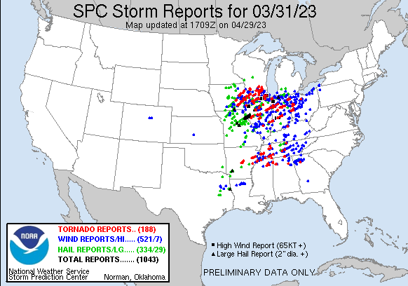
This exercise walks through the steps of setting up and running a WRF simulation for a single domain. The case used for this test is a severe storm outbreak over the midwest and southest United States. The case takes place from 31 March to 1 April, 2023. There were over 1000 severe storm reports that included 188 tornado reports.
Note
Since this is a single domain run, max_dom is set to 1, and therefore the WPS programs will only read the first column. DO NOT remove settings for additional columns! Just simply change the settings for column 1.
See WPS Namelist Variables from the WRF Users’ Guide for details about each parameter.
See namelist.wps Best Practices for additional information and suggestions.
Run the Geogrid Program
The geogrid program defines the map projection, as well as the geographic location, size, and resolution of the domain. It also interpolates static fields (e.g., topography height, landuse category, etc.) to the domain.
Follow the steps below to configure the domain and create static files for the specific domain.
If the static geographic files have not already been downloaded, do this first. Unpack the file in a unique directory (e.g., in a directory called WPS_GEOG). Make sure to download the file for the “Highest Resolution of Each Mandatory Field.”
Move to the WPS directory.
Edit namelist.wps in the top-level WPS directory. Make changes to incorporate the following settings:
&share
max_dom = 1,

&geogrid
parent_id = 1,
parent_grid_ratio = 1,
i_parent_start = 1,
j_parent_start = 1,
e_we = 100,
e_sn = 100,
geog_data_res = 'default'
dx = 30000
dy = 30000
map_proj = 'lambert',
ref_lat = 38
ref_lon = -90
truelat1 = 30.0
truelat2 = 60.0
stand_lon = -90
geog_data_path = 'path-to-static-files'
Note
Only some namelist variables require settings for both domains. If there is only a single setting for a variable in the default namelist (or in the list above), do not add another column - it will give an error when you try to run.
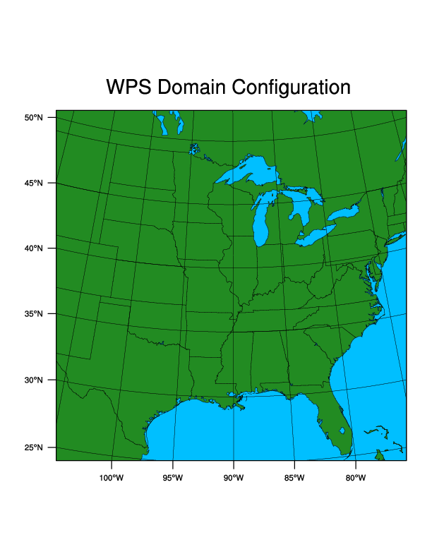
Check that the domain is in the correct location using the NCL plotgrids script, available in the WPS/util directory.
ncl util/plotgrids_new.ncl
If x-forwarding is installed, a window should pop up to the desktop with an image of the domain. It should look like the following:
Run geogrid to create static data files for this specific domain.
./geogrid.exe
Text will print to the screen as geogrid processes. Look for the following at the end of the prints:
!!!!!!!!!!!!!!!!!!!!!!!!!!!!!!!!!!!!!!!!!!!!!
! Successful completion of geogrid.         !
!!!!!!!!!!!!!!!!!!!!!!!!!!!!!!!!!!!!!!!!!!!!!
There should now be a geo_em.d01.nc file available in the WPS directory. This is the output from the geogrid program. It it is not successful, see the geogrid.log file created during the geogrid execution. Try to troubleshoot the errors. If unable to do so, see the WRF & MPAS-A User Support Forum to search for previous solutions to the issue, and if unable to find anything, post a new thread to the forum.
Feel free to look at the contents of the geo_em.d01.nc file.
Use the netCDF ncdump utility:
ncdump -h geo_em.d01.nc
Use the netCDF data browser, ncview, to view field images from the file:
ncview geo_em.d01.nc
Run the Ungrib Program
Input meteorological data are often in GRIB format. The ungrib program reads these data, extracts the meteorological fields, and then writes those fields to an intermediate file format that can be read by the next program (metgrid).
Follow the steps below to convert grib-formatted input meteorological data to an intermediate format expected by the metgrid program.
The data used for this case are final analysis data from the NCEP GFS model. These GRIB2-formatted data files have a temporal resolution of six hours and a horizontal resolution of one degree. There are 34 pressure levels available. Note that higher resolution are available from the GFS model, but for the purpose of learning, coarse data are okay to use.
Create a unique directory in which to place the input data (e.g., data). Download 3d and surface GFS data for this case and unpack the files in the newly-created directory.
mkdir data

cd data

tar -xf severe_outbreak.tar.gz
Note
Feel free to use the g2print.exe program from the WPS/util directory to look at the raw data. From the WPS directory, use the command
./util/g2print.exe path-to-data-files/fnl_20230331_00_00.grib2Link the meteorological input files to the WPS directory using the link_grib.csh script available in the top-level WPS directory. Note that the files (and not just the directory containing the files) should be linked, but only the prefix is necessary. There is also no need to specify the files should be put “here” (or “.”) - this is built into the script.
./link_grib.csh path-to-input-data/fnl
After this, issue
ls -ls GRIBFILE*to see the following files are now linked to the WPS directory. The files are in the format of GRIBFILE.XXX and there is one file per input data file (time period). These files are linked back to the original files.GRIBFILE.AAA -> path-to-input-data/fnl_20230331_00_00.grib2 GRIBFILE.AAA -> path-to-input-data/fnl_20230331_06_00.grib2 GRIBFILE.AAA -> path-to-input-data/fnl_20230331_12_00.grib2 GRIBFILE.AAA -> path-to-input-data/fnl_20230331_18_00.grib2 GRIBFILE.AAA -> path-to-input-data/fnl_20230401_00_00.grib2
Link the GFS Vtable to the WPS directory, as the generic name “Vtable.” which is the name expected by the ungrib program.
ln -sf ungrib/Variable_Tables/Vtable.GFS Vtable
Now, issue
ls -lsto see the file “Vtable” linked back to the GFS Vtable.Note
Feel free to take a look at the Vtable to see which fields are going to be processed.
Edit namelist.wps in the top-level WPS directory. Make changes to incorporate the following settings:
&share
max_dom = 1
start_date = '2023-03-31_00:00:00 ',
end_date = '2023-04-01_00:00:00 ',
interval_seconds = 21600

&ungrib
prefix = 'FILE',
Run ungrib to convert the GRIB2 files to intermediate file format.
./ungrib.exe
Look for the following text printed to the screen when ungrib completes.
!!!!!!!!!!!!!!!!!!!!!!!!!!!!!!!!!!!!!!!
!  Successful completion of ungrib.   !
!!!!!!!!!!!!!!!!!!!!!!!!!!!!!!!!!!!!!!!
The files in intermediate format should now be available in the WPS directory. They are in the format of FILE:YYYY-MM-DD_hh for each time. If ungrib does not run successfully, see the ungrib.log file created during the ungrib process. Try to troubleshoot the errors. If unable to do so, see the WRF & MPAS-A User Support Forum to search for previous solutions to the issue, and if unable to find anything, post a new thread to the forum.
Feel free to look at the contents of the intermediate files using the rd_intermediate.exe program available in the WPS/util directory. For e.g.,
./util/rd_intermediate.exe FILE:2023-03-31_00
Run the Metgrid Program
The metgrid program horizontally interpolates meteorological data (extracted by the ungrib program) to simulation domains (defined by geogrid), and creates the input data files necessary to run the WRF model.
Follow the below steps to horizontally interpolate the meteorological input data onto the model domain using the output from geogrid (geo_em.d01.nc) and the intermediate formatted files from ungrib (FILE:*)
No namelist.wps modifications are required for running metgrid in this case. Just ensure the dates and times are set correctly, and that the variable fg_name is set to FILE so it is able to find the intermediate files.
Run metgrid.exe
./metgrid.exe
Text will print to the screen as metgrid processes. Look for the following at the end of the prints.
!!!!!!!!!!!!!!!!!!!!!!!!!!!!!!!!!!!!!!!
!  Successful completion of metgrid.  !
!!!!!!!!!!!!!!!!!!!!!!!!!!!!!!!!!!!!!!!
If successful, metgrid output in the format of met_em.d01.YYYY-MM-DD_hh:mm:ss.nc will be available in the top-level WPS directory. There should be one file per time period.
Feel free to look at the contents of the met_em files.
Use the netCDF ncdump utility. For e.g.,
ncdump -h met_em.d01.2023-03-31_00:00:00.nc
Use the netCDF data browser, ncview, to view field images from the files; for e.g.,
ncview met_em.d01.2023-03-31_00:00:00.nc
Run the Real Program
The real.exe program defines the WRF model vertical coordinate. It uses horizontally-interpolated meteorological data (met_em* files from wps) and vertically interpolates them for use with the WRF model. It creates initial condition files and a lateral boundary file that will be used by WRF.
Follow the steps below to vertically interpolate the input data to the model coordinates.
Move to the WRF/test/em_real directory.
Link the metgrid output files to the em_real directory.
ln -sf path-to-WPS/met_em* .
Edit namelist.input available in the em_real directory. Make changes to incorporate the following settings:
Note
Since this is a single domain run, max_dom is set to 1, and therefore the real and wrf programs will only read the first column. DO NOT remove settings for additional columns! Just simply change the settings for column 1.
See WRF Namelist Variables from the WRF Users’ Guide for details about each parameter.
See namelist.input Best Practices for additional information and suggestions.
&time_control
run_hours = 24,
run_minutes = 0,
start_year = 2023,
start_month = 03,
start_day = 31,
start_hour = 00,
end_year = 2023,
end_month = 04,
end_day = 01,
end_hour = 00
interval_seconds = 21600
input_from_file = .true.
history_interval = 180,
frames_per_outfile = 1,
restart = .false.,
restart_interval = 720,

&domains
time_step = 150
max_dom = 1,
e_we = 100,
e_sn = 100,
e_vert = 45,
num_metgrid_levels = 34
num_metgrid_soil_levels = 4
dx = 30000
dy = 30000
Note
The restart_interval parameter tells the model to create a restart file every 720 hours. This will be used later for the Restart Case.
The num_metgrid_levels setting of 34 and the num_metgrid_soil_levels setting of 4 comes from the meteorological input data. To see the correct settings for this with future data, use the command
ncdump -h met_em.d01.YYYY-MM-DD_hh:mm:ss.nc(for one of the met_em) files and look for the values.
Run real.exe.
Depending on how WRF was installed (e.g., for serial or dmpar computation), the command to run real.exe will differ. Additionally, if using dmpar (parallel processing) on a cluster, it is possible a batch script is required to submit the command. Within that batch script, the same type of MPI command will be used. Use something similar to the following (it may be necessary to ask a systems administrator at your institution for guidance on the proper command for your machine/environment).
For parallel-processing (dmpar)
mpiexec -np X ./real.exe
The X here indicates the number of processors to use. real.exe is a quick process and probably does not need a lot of processors - especially for this fairly small simulation. An appropriate number would be somewhere between ~1-50.
For serial processing (using a single processor)
./real.exe >& real.log
The error and output will go to the real.log file for serial computation, and for parallel computation, there will be an rsl.out and rsl.error file available for each processor. Check the end of those files for the “SUCCESS” message to ensure real.exe ran correctly. If successful, the output files wrfbdy_d01 and wrfinput_d01 will be available in the em_real directory.
Run the WRF Model
The WRF model uses the intitial and boundary condition files generated by the real program to perform model integration, using user-specified options provided in the namelist.input file (e.g., physics options).
Run wrf.exe
Just as with real.exe, depending on how WRF was installed (e.g., for serial or dmpar computation), the command to run wrf.exe will differ.
For parallel-processing (dmpar)
mpiexec -np X ./wrf.exe
The X here indicates the number of processors to use. An appropriate number of processors for this particular simulation would be somewhere between ~1-50. wrf.exe is a more computationally-intensive process than real, so the number of processors matters more. See Choosing an Appropriate Number of Processors.
For serial processing (using a single processor)
./wrf.exe >& wrf.log
The error and output will go to the wrf.log file for serial computation, and for parallel computation, there will be an rsl.out and rsl.error file available for each processor. Check the end of those files for the “SUCCESS” message to ensure wrf.exe ran correctly. If successful, the output files wrfout_d01_YYYY-MM-DD_hh:mm:ss will be available in the em_real directory.
Since history_interval=180 in the namelist, this means that history is printed out every three hours, and because frames_per_outfile=1, there will be one file per history_interval. This means there should be eight total wrfout files, starting with the initial time of the simulation.
Note
In addition to the wrfout files, there will be wrfrst_d01 files output. Because restart_interval=720 in the namelist, a restart file is output every 12 hours, meaning there should be two wrfrst_d01 files available in the em_real directory. These files will be used and discussed later in the Restart Case.
To look at the contents in the wrfout files, use either the netCDF ncdump utility, or the ncview tool.