The Adaptive Time-step Option

This exercise teaches the use of the Adaptive Time Stepping option, instead of a fixed time step.

Adaptive Time Stepping

A method to maximize the time step when the model timestep time_step must be reduced to maintain model stability. This option can allow the model to run faster, overall. It is typically used in real-time or climate model runs.

If you have existing wrfinput_d01 and wrfbdy_d01 files from the Single Domain Run, WPS pre-processing can be skipped. If not, return to the Single Domain exercise and generate these files again.

1. Add the following to the &domains record in namelist.input.

   
   

   &domains
   max_dom = 1
   use_adaptive_time_step  = .true.,
   step_to_output_time     = .true.,
   target_cfl              = 1.2, 1.2,
   target_hcfl             = .84, .84,
   max_step_increase_pct   = 5, 51,
   starting_time_step      = -1, -1,
   max_time_step           = 240, 240,
   min_time_step           = 120, 120,
   adaptation_domain       = 1,
   

   
   

   Note

   • Recommended min and max time steps are \(3 \times dx\) and \(8 \times dx\), respectively.

   • It’s important that the min and max are not so far apart that the model time steps drastically vary.

   • Since max_dom=1, the model will only read the first namelist column, but we display two columns above to demonstrate which variables require a setting for each domain.

   
   

2. It’s not necessary to run real.exe again, just run wrf.exe.

Check your output

When using fixed time steps the rsl.out.0000 file includes prints like the following, showing the elapsed time for each fixed model time step:

Timing for main: time 2023-03-31_00:03:00 on domain 1: 3.43441 elapsed seconds
Timing for main: time 2023-03-31_00:06:00 on domain 1: 2.11485 elapsed seconds
Timing for main: time 2023-03-31_00:09:00 on domain 1: 2.05235 elapsed seconds
Timing for main: time 2023-03-31_00:12:00 on domain 1: 2.16914 elapsed seconds
Timing for main: time 2023-03-31_00:15:00 on domain 1: 2.05815 elapsed seconds
Timing for main: time 2023-03-31_00:18:00 on domain 1: 2.17894 elapsed seconds
Timing for main: time 2023-03-31_00:21:00 on domain 1: 2.07029 elapsed seconds
Timing for main: time 2023-03-31_00:24:00 on domain 1: 2.18028 elapsed seconds
Timing for main: time 2023-03-31_00:27:00 on domain 1: 2.09054 elapsed seconds
Timing for main: time 2023-03-31_00:30:00 on domain 1: 2.19225 elapsed seconds

When using adaptive time step, the length of the time step is also included. Note that although the time_step starts lower, they quickly become longer than the original dt=150 used for the fixed time step runs. Because step_to_output_time=.true., the model outputs every 3 hours, on the hour.

Timing for main (dt=120.00): time 2023-03-31_00:02:00 on domain 1: 1.43449 elapsed seconds
Timing for main (dt=126.00): time 2023-03-31_00:04:06 on domain 1: 0.07998 elapsed seconds
Timing for main (dt=132.30): time 2023-03-31_00:06:18 on domain 1: 0.08054 elapsed seconds
Timing for main (dt=138.91): time 2023-03-31_00:08:37 on domain 1: 0.08064 elapsed seconds
Timing for main (dt=145.86): time 2023-03-31_00:11:03 on domain 1: 0.08072 elapsed seconds
Timing for main (dt=153.15): time 2023-03-31_00:13:36 on domain 1: 0.08088 elapsed seconds
Timing for main (dt=160.81): time 2023-03-31_00:16:17 on domain 1: 0.08190 elapsed seconds
Timing for main (dt=168.85): time 2023-03-31_00:19:05 on domain 1: 0.43627 elapsed seconds
Timing for main (dt=177.29): time 2023-03-31_00:22:03 on domain 1: 0.08504 elapsed seconds
Timing for main (dt=186.15): time 2023-03-31_00:25:09 on domain 1: 0.08125 elapsed seconds
Timing for main (dt=195.46): time 2023-03-31_00:28:24 on domain 1: 0.08498 elapsed seconds
Timing for main (dt=205.23): time 2023-03-31_00:31:50 on domain 1: 0.08544 elapsed seconds

To plot the model time steps, copy the appropriate NCL script to your wrf/test/em_real directory. This script is already edited for this case, but before running it, use the below “grep” command to obtain the time steps from rsl.out.0000.

cp WRF_NCL_scripts/wrf_AdaptiveTime.ncl .

grep "Timing for main" rsl.out.0000 > adaptive_times.txt

ncl wrf_AdaptiveTime.ncl

This following plot should be created:

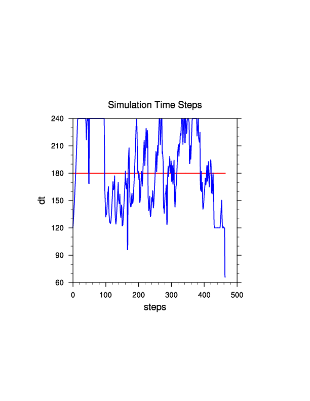
• The red line represents a constant time of 180 seconds.

• The blue line represents the actual time steps the model took.

It is clear the model mostly took time steps larger than 180 seconds. Notice the occasional big drops in time steps. This is not desirable. For this case we could easily set the minimum time step to 200 seconds, as the model takes bigger time steps the entire time. We want to prevent big drops and large differences in time steps, so setting the maximum time step to no more than 360 would be more sensible than our test setting of 420.

What is in the NCL script?

Reading data
To read and use the data from text files, you need to know a bit about the file. The data are a mix between characters and numbers and not simple to interpret. So we are going to read the data with the NCL systemfunc function rather than with typical NCL read commands.

tmp = systemfunc("cut -c21-26 adaptive_times.txt")

Note that we need to read characters 21-26 (so some counting is in order).

Plotting the data
We need three pieces of information for plotting:

1. An \(x\) coordinate, which is created as a simple 0 to \(n\) array (steps)

2. A constant 180 second line, which we place in data(0,:)

3. The actual time steps the model took, which we place in data(1,:)

Note the tmp array we read consists of characters. We need to convert this to floats before plotting (stringtofloat)

plot = gsn_csm_xy(wks,steps,data,res)

Return to the Practice Exercise home to page to run the Single Domain Run.

• Return to Practice Exercises