Set-up and Run Your Own Case
This exercise allows you to set up and run WPS and WRF, but instead of us dictating your case setup, you can be creative and play around with domains.
Important
For your job- or school-related purpose, high resolution and larger number of grid points may be required, but to respect this class’s shared computation limits, for this exercise, please use resolution and sizes similar to those in previous exercises. The purpose is to become familiar with the steps and considerations needed to make your own case - not the actual size of the problem.
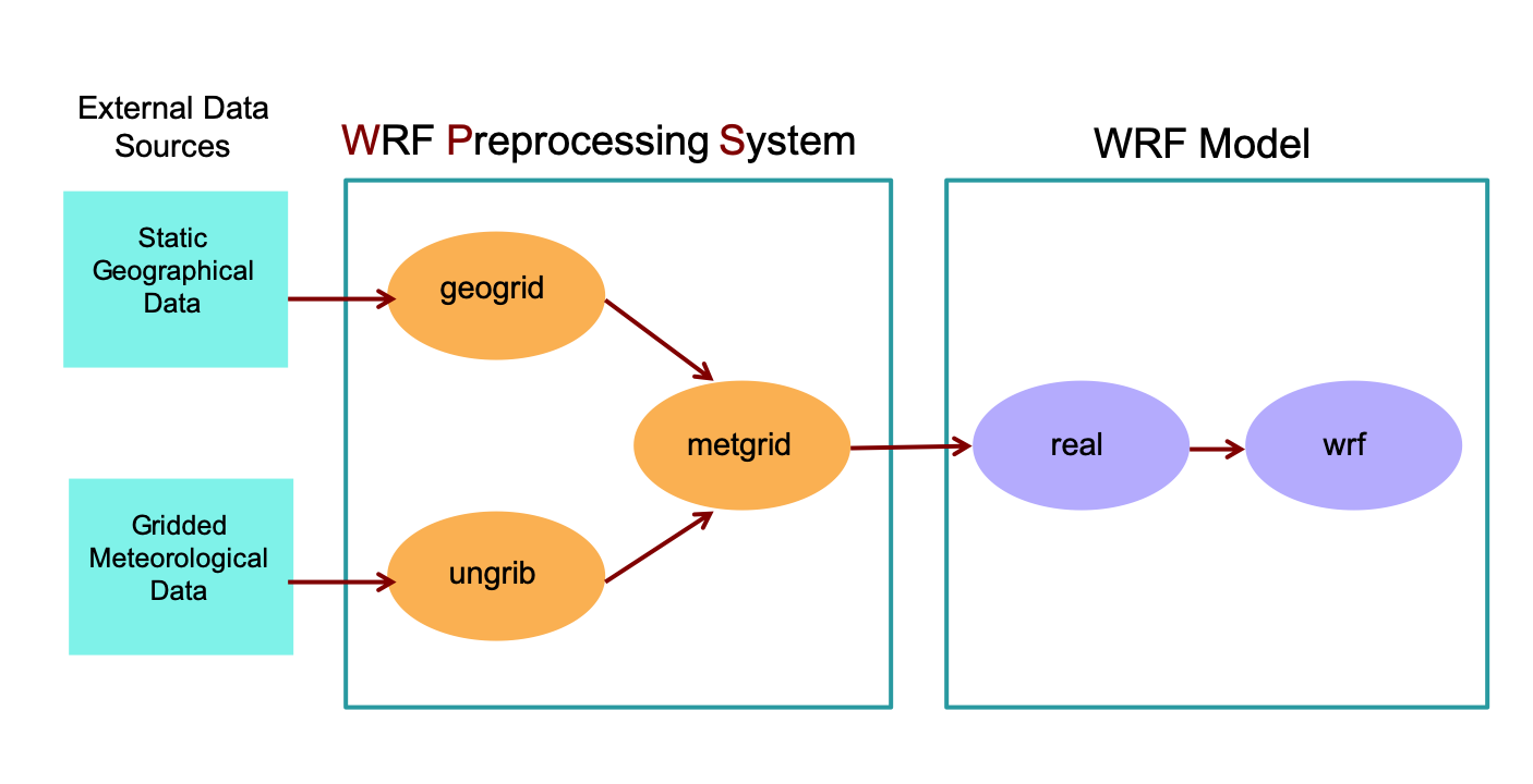
Follow the five below processes. Run the WPS processes in the wps directory, and run real and wrf in the wrf/test/em_real directory.
Download Input Data
You may use any GRIB-formatted meteorological data you have access to, or use one of the following options to obtain data:
Use any dataset provided for the tutorial exercises - noting that these are available for specific dates/times.
Colorado Blizzard (Nov 2019) Global Data
/glade/campaign/mmm/wmr/wrf_tutorial/input_data/colorado_blizzard/fnl_2021March-April 2023 Severe Weather Outbreak Global Data
/glade/campaign/mmm/wmr/wrf_tutorial/input_data/severe_outbreak/fnl_20230Hurricane Matthew (Oct. 2016) Global Data
/glade/campaign/mmm/wmr/wrf_tutorial/input_data/matthew/gfs.0p25.2016100October 2016 Global Data
/glade/campaign/mmm/wmr/wrf_tutorial/input_data/climate_cfsv2/cdas1.2016100Two different Vtables are required for these data (see the Climate Simulation for details).
Real-time GFS forecast data. These are only available for a short period of time, so use a time period in the past few days.
See available GRIB Datasets from NSF NCAR’s data archives for free input data. All data types are available in /glade/campaign/collections/rda/data/ds* (where ds* is the data type number).
Geogrid
Edit namelist.wps to configure the domain using options such as e_we/e_sn/i_parent_start/j_parent_start/dx/dy to specify grid size and placement. If you want a nest, make appropriate namelist changes for multiple domains. Consider the following:
Are nested domains required to reach the target resolution?
Are there any potential problems with boundary locations?
How long will it take a typical air parcel to pass from one side of the domain to the other (consider the importance of domain size)?
Based on other exercises, roughly how computationally expensive will this domain configuration be, and how long will this simulation take?
Use util/plotgrids_new.ncl to visualize your domain. Play with namelist settings until the domain is right. If using a nest, it may be useful to first visualize the coarse domain, and once satisfied, use the visualiztion tool to outline the nest domain (i.e., to find the child domain’s starting and ending endices). Then compute the nest’s number of grid points.
Run geogrid.
Ungrib
Modify the namelist dates, set interval_seconds to reflect the number of seconds between your data intervals.
Link the GRIB data into the wps directory.
Link-in the correct Vtable.
Run ungrib to generate intermediate files.
Metgrid
Run metgrid to create the met_em.d0* files for the real.exe program.
Real & WRF
Modify case domain and date information in namelist.input. Use lessons from previous exercises to determine what other variables need to be modified.
Link-in the appropriate files and then run real and wrf.
View the rsl.out* files to ensure the run was successful. If you wish, view some of your data with the available graphics options.
Return to the Practice Exercise home to page to run another exercise.