Two-way Nested Domain¶

A two-way nested simulation uses two or more domains. A parent (coarse) domain contains one or more finer-resolution domains. The domains run simultaneously and communicate - the coarser domain provides boundary values to the nest, and if the namelist.input parameter feedback is turned on (=1), the nest feeds its calculations back to the coarse domain.

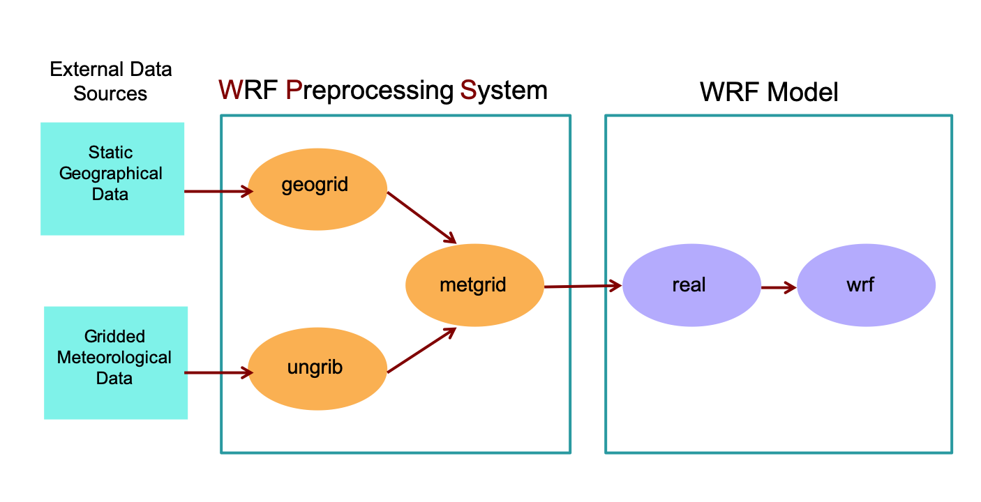
WPS: Geogrid¶

Recall that the geogrid program interpolates static fields to the user-defined domain. Now do this for 2 domains.**

Move to the wps directory.
Edit namelist.wps to configure the simulation domain. Highlighted modifications in the box below are specific to including a nested domain.

Note

To avoid errors, do not add additional columns/entries for namelist variables with only a single setting. If the default namelist only has a single value, the model only expects a single value.

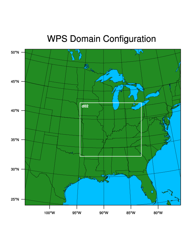
Add a nested domain over the midwest United States, using the following specifications:
- 118 x103 grid points
- a 3:1 grid ratio between the second and first domains
Make the following changes to the &share and &geogrid records in namelist.wps.
```
     &share
     max_dom = 2,

     &geogrid
     parent_id = 1, 1,
     parent_grid_ratio = 1, 3,
     i_parent_start = 1, 36
     j_parent_start = 1, 32
     e_we = 100, 118
     e_sn = 100, 103
     dx = 30000
     dy = 30000
     geog_data_res = 'default','default',
     geog_data_path = '/glade/work/wrfhelp/WPS_GEOG'
```
Note

To determine appropriate e_we and e_sn settings for domain 2, the following equation must result in a whole number: \((dimension - 1) \div parent\_grid\_ratio\). Use the above example to check the e_we setting:
- \(dimension = 118\)
- \(1\) is subtracted because there is one additional velocity point (grid edges) per direction, than grid cells
- \(parent\_grid\_ratio = 3\) since there is a 3:1 ratio between d02 and d01
The resulting value is \(x=39\), which is, indeed, a whole number, and therefore setting e_we = 118 is okay for d02. If interested, test for the value of e_sn.
Preview the domain to make sure it is correct.
Now generate geographical data files geo_em.d01.nc and geo_em.d02.nc by running geogrid.exe

DO NOT Run Ungrib¶

Recall that the ungrib program converts meteorological data input from GRIB to intermediate format. Because data are specific to the date and time of the simulation, and are not domain-dependent, if you already have the intermediate files (prefix FILE) from the Single Domain Run, there is no need to rerun the ungrib program. You may continue to run metgrid. If you no longer have these files, go back to the Single Domain Run and repeat step 2.

WPS: Metgrid¶

Recall that the metgrid program horizontally interpolates meteorological data to the simulation domains. Run metgrid to do this on both domains.

Ensure the domain 2 dates/times are correct in namelist.wps.
```
&share
start_date = '2023-03-31_00:00:00 ', '2023-03-31_00:00:00 ',
end_date = '2023-04-01_00:00:00 ', '2023-03-31_00:00:00 ',
interval_seconds = 21600 ,
```
Note

If you’re not using nudging or SST-update options, end_date for domain 2 can be equal to the start_date. Only the initial time is required for nested domains because they receive boundary conditions from d01.
Run metgrid.exe to create the following files - note the single domain 2 file:

met_em.d01.2023-03-31_00:00:00.nc
met_em.d01.2023-03-31_06:00:00.nc
met_em.d01.2023-03-31_12:00:00.nc
met_em.d01.2023-03-31_18:00:00.nc
met_em.d01.2023-04-01_00:00:00.nc
met_em.d02.2023-03-31_00:00:00.nc
If interested, use ncview to view the metgrid output.

Prep for Real & WRF¶

Move to the wrf/test/em_real directory.

Edit namelist.input to reflect domain and date information for this case, and to include settings for domain 02.

Important

Remember - do not remove or add any columns. Just modify those that exist.

     &time_control
     run_hours = 24,
     start_year = 2023, 2023,
     start_month = 03, 03,
     start_day = 31, 31,
     start_hour = 00, 00,
     end_year = 2023, 2023,
     end_month = 04, 04,
     end_day = 01, 01,
     end_hour = 00, 00
     interval_seconds = 21600
     input_from_file = .true.,.true.,
     history_interval = 180, 180,
     frames_per_outfile = 1, 1,
     restart = .false.,
     restart_interval = 72000,

     &domains
     time_step = 150
     max_dom = 2,
     e_we = 100, 118
     e_sn = 100, 103
     e_vert = 45, 45,
     num_metgrid_levels = 34
     num_metgrid_soil_levels = 4
     dx = 30000
     dy = 30000
     grid_id = 1, 2,
     parent_id = 0, 1,
     i_parent_start = 1, 36
     j_parent_start = 1, 32
     parent_grid_ratio = 1, 3,
     parent_time_step_ratio = 1, 3,

Note

When uncertain which namelist parameters require a single setting (not domain-specific), or settings per domain (multiple columns), see the parameter’s registry setting (found in wrf/Registry/* files - typically in Registry.EM_COMMON). The “Nentries” column indicates either max_domains (meaning a setting is required per domain) or 1 (only a single domain-independent setting allowed).
input_from_file=.true.,.true. creates input data files (wrfinput_d01 and wrfinput_d02), which is standard for basic nested cases. When running the vortex-following case, you will set input_from_file=.true.,.false.

Run Real¶

Recall the real program uses horizontally-interpolated meteorological data (met_em* files) and vertically interpolates them to create initial and boundary conditions that are used to run the wrf model.

Link the metgrid output from wps to the current directory.
Submit the runreal.sh batch script to the queue to run real.exe and produce the following files. Note: no wrfbdy_d02 file is created because nests obtain boundary conditions from their parent):

wrfbdy_d01
wrfinput_d01
wrfinput_d02

View rsl.out.0000 to ensure the process was successful.

Run WRF¶

Recall the WRF model uses intitial and boundary conditions generated by the real program and user-specified namelist.input options to perform model integration.

Submit the runwrf.sh batch script to the queue to run the nested wrf simulation.

Running a 24-hour simulation for this 2-domain case could take ~10 mins to complete. Use the qstat command to check your simulation’s status, or see rsl.out.0000. If successful, the following history files are generated:

wrfout_d01_2023-03-31_00:00:00
wrfout_d01_2023-03-31_03:00:00
wrfout_d01_2023-03-31_06:00:00
wrfout_d01_2023-03-31_09:00:00
wrfout_d01_2023-03-31_12:00:00
wrfout_d01_2023-03-31_15:00:00
wrfout_d01_2023-03-31_18:00:00
wrfout_d01_2023-04-01_00:00:00

wrfout_d02_2023-03-31_00:00:00
wrfout_d02_2023-03-31_03:00:00
wrfout_d02_2023-03-31_06:00:00
wrfout_d02_2023-03-31_09:00:00
wrfout_d02_2023-03-31_12:00:00
wrfout_d02_2023-03-31_15:00:00
wrfout_d02_2023-03-31_18:00:00
wrfout_d02_2023-04-01_00:00:00

Feel free to use some of the options or graphics mentioned in previous exercises to view your output.

Return to the Practice Exercise home to page to run another exercise.

Return to Practice Exercises