Output Time Series Data
Generate time series output at specific station locations within your domain to see the progression of certain variables.
See also
See wrf/run/README.tslist for additional details.
If wrfinput_d01 and wrfbdy_d01 from the Initial Exercise (initial_exercise) are available, no data pre-processing is needed; copy them to your wrf running directory. Otherwise recreate those files to run this case.
cp initial_exercise/namelist.input .
cp initial_exercise/wrfbdy_d01 .
cp initial_exercise/wrfinput_d01 .
Create the input text file containing station information. WRF expects a tslist text file in the running directory. To ensure correct formatting, copy a pre-made tslist to your running directory:
cp /glade/campaign/mmm/wmr/wrf_tutorial/tslist .
The content of the file is as follows:
#-----------------------------------------------#
# 24 characters for name | pfx  | LAT   | LON   |
#-----------------------------------------------#
Boulder                    kbou  40.000  -105.150
Broomfield                 kbjc  39.550  -105.070
Denver Airport             kden  39.490  -104.390
No need to re-run real.exe. Run wrf.exe using the “runwrf_initial.sh” script. If successful, the following time series output files will be generated - one set per each pfx specified in tslist.
kbou.d01.PH kbjc.d01.PH kden.d01.PH kbou.d01.PR kbjc.d01.PR kden.d01.PR kbou.d01.QV kbjc.d01.QV kden.d01.QV kbou.d01.TH kbjc.d01.TH kden.d01.TH kbou.d01.TS kbjc.d01.TS kden.d01.TS kbou.d01.UU kbjc.d01.UU kden.d01.UU kbou.d01.VV kbjc.d01.VV kden.d01.VV kbou.d01.WW kbjc.d01.WW kden.d01.WW
The pfx*.dNN.TS file contains time series of surface variables at each time step, while all other files contain vertical profile data for geopotential height, potential temperature, water vapor mixing ratio, and wind, at each time step.
Check your output
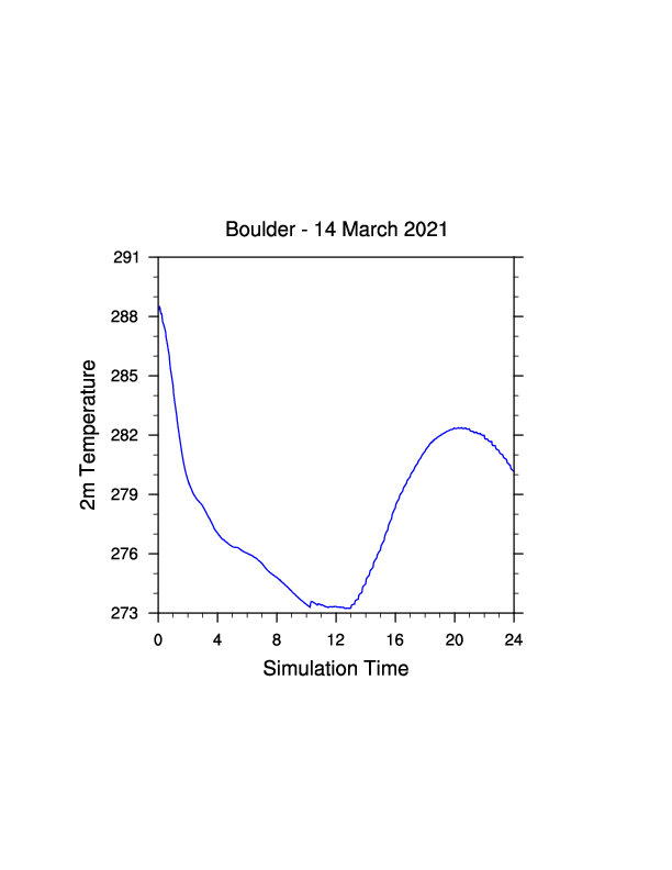
Plot a time series of surface temperature at the Boulder station.
From test/em_real, copy in, and run, the appropriate NCL script, which is already edited for this case.
WRF_NCL_scripts/wrf.ts.ncl .

ncl wrf.ts.ncl
The following plot should appear:
If desired, plot a different variable (e.g., surface pressure), using the same NCL script - but you will need to make some modifications. Use the following to guide your modifications:
Reading data
Note that the file kbou.d01.TS contains 19 columns of real/float data, with one header record.
Therefore the NCL function readAsciiTable can be used to read the data.
data = readAsciiTable("kbou.d01.TS", 19, "float", 1)
Plotting the data
First you must set some plot resources considering the following:
The first column in the file is a domain I.D.
The second is the forecast hour
The 6th record is 2m temperature
To plot temperature over time you need columns 2 and 6 (this will be 1 and 5 in NCL). Plot the data using:
plot = gsn_csm_xy(wks,data(:,1),data(:,5),res)
Return to the Practice Exercise home to page to run another exercise.